Hessian and Basin volume
2Thomas Larsen
1Charlie Steiner
1Thomas Larsen
4Vivek Hebbar
0Charlie Steiner
1Thomas Kwa
4Vivek Hebbar
New Comment
I am a bit confused how you deal with the problem of 0 eigenvalues in the Hessian. It seems like the reason that these 0 eigenvalues exist is because the basin volume is 0 as a subset of parameter space. My understanding right now of your fix is that you are adding along the diagonal to make the matrix full rank (and this quantity is coming from the regularization plus a small quantity). Geometrically, this seems like drawing a narrow ellipse around the subspace of which we are trying to estimate the volume.
But this doesn't seem natural to me, seems to me like the most important part of determining volume of these basins is the relative dimensionality. If there are two loss basins, but one has dimension greater than the other, the larger one dominates and becomes a lot more likely. If this is correct, we only care about the volume of basins that have the same number of dimensions. Thus, we can discard the dimensions with 0 eigenvalue and just apply the formula for the volume over the non-zero eigenvalues (but only for the basins with maximum rank hessians). This lets us directly compare the volume of these basins, and then treat the low dimensional basins as having 0 volume.
Does this make any sense?
The hessian is just a multi-dimensional second derivative, basically. So a zero eigenvalue is a direction along which the second derivative is zero (flatter-bottomed than a parabola).
So the problem is that estimating basin size this way will return spurious infinities, not zeros.
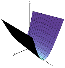
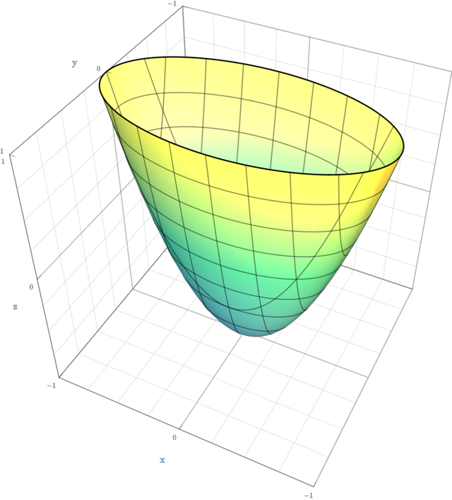
Thanks for your response! I'm not sure I communicated what I meant well, so let me be a bit more concrete. Suppose our loss is parabolic , where . This is like a 2d parabola (but it's convex hull / volume below a certain threshold is 3D). In 4D space, which is where the graph of this function lives and hence where I believe we are talking about basin volume, this has 0 volume. The hessian is the matrix:
This is conveniently already diagonal, and the 0 eigenvalue comes from the component , which is being ignored. My approach is to remove the 0-eigenspace, so we are working just in the subspace where the eigenvalues are positive, so we are left with just the matrix: , after which we can apply the formula given in the post:
If this determinant was 0 then dividing by 0 would get the spurious infinity (this is what you are talking about, right?). But if we remove the 0-eigenspace we are left with positive volume, and hence avoid this division by 0.
The loss is defined over all dimensions of parameter space, so is still a function of all 3 x's. You should think of it as . It's thickness in the direction is infinite, not zero.
Here's what a zero-determinant Hessian corresponds to:

The basin here is not lower dimensional; it is just infinite in some dimension. The simplest way to fix this is to replace the infinity with some large value. Luckily, there is a fairly principled way to do this:
- Regularization / weight decay provides actual curvature, which should be added in to the loss, and doing this is the same as adding to the Hessian.
- The scale of the initialization distribution provides a natural scale for how much volume an infinite sweep should count as (very roughly, the volume only matters if it overlaps with the initialization distribution, and the distance of sweep for which this is true is on the order of , the standard deviation of the initialization).
So the is a fairly principled correction, and much better than just "throwing out" the other dimensions. "Throwing out" dimensions is unprincipled, dimensionally incorrect, numerically problematic, and should give worse results.
Note that this is equivalent to replacing "size 1/0" with "size 1". Issues with this become apparent if the scale of your system is much smaller or larger than 1. A better try might be to replace 0 with the average of the other eigenvalues, times a fudge factor. But still quite unprincipled - maybe better is to try to look at higher derivatives first or do nonlocal numerical estimation like described in the post.
Do you have thoughts on when there are two algorithms that aren’t “doing the same thing” that fall within the same loss basin?
It seems like there could be two substantially different algorithms which can be linearly interpolated between with no increase in loss. For example, the model is trained to classify fruit types and ripeness. One module finds the average color of a fruit (in an arbitrary basis), and another module uses this to calculate fruit type and ripeness. The basis in which color is expressed can be arbitrary, since the second module can compensate.
- Here, there are degrees of freedom in specifying the color basis and parameters can probably be eliminated, but it would be more interesting to see examples where two semantically different algorithms fall within the same basin without removable degrees of freedom, either because the Hessian has no zero eigenvalues, or because parameters cannot be removed despite the Hessian having a zero eigenvalue.
From this paper, "Theoretical work limited to ReLU-type activation functions, showed that in overparameterized networks, all global minima lie in a connected manifold (Freeman & Bruna, 2016; Nguyen, 2019)"
So for overparameterized nets, the answer is probably:
- There is only one solution manifold, so there are no separate basins. Every solution is connected.
- We can salvage the idea of "basin volume" as follows:
- In the dimensions perpendicular to the manifold, calculate the basin cross-section using the Hessian.
- In the dimensions parallel to the manifold, ask "how can I move before it stops being the 'same function'?". If we define "sameness" as "same behavior on the validation set",[1] then this means looking at the Jacobian of that behavior in the plane of the manifold.
- Multiply the two hypervolumes to get the hypervolume of our "basin segment" (very roughly, the region of the basin which drains to our specific model)
- ^
There are other "sameness" measures which look at the internals of the model; I will be proposing one in an upcoming post.
Curated and popular this week
