All of Logan Riggs's Comments + Replies

A weird example of this is on page 33 (full transcript pasted farther down) 

tl;dr: It found a great general solution for speeding up some code on specific hardward, tried to improve more, resorted to edge cases which did worse, and submitted a worse version (forgetting the initial solution).

This complicates the reward hacking picture because it had a better solution that got better reward than special-casing yet it still resorted to special-casing. Did it just forget the earlier solution? Feels more like a contextually activated heuristic to special-c... (read more)

Thinking through it more, Sox2-17 (they changed 17 amino acids from Sox2 gene) was your linked paper's result, and Retro's was a modified version of factors Sox AND KLF. Would be cool if these two results are complementary.

You're right! Thanks
For Mice, up to 77% 

Sox2-17 enhanced episomal OKS MEF reprogramming by a striking 150 times, giving rise to high-quality miPSCs that could generate all-iPSC mice with up to 77% efficiency

For human cells, up to 9%  (if I'm understanding this part correctly).
 

SOX2-17 gave rise to 56 times more TRA1-60⁺ colonies compared with WT-SOX2: 8.9% versus 0.16% overall reprogramming efficiency.

So seems like you can do wildly different depending on the setting (mice, humans, bovine, etc), and I don't know what the Retro folks were doing, but does make their result less impressive. 

For those also curious, Yamanaka factors are specific genes that turn specialized cells (e.g. skin, hair) into induced pluripotent stem cells (iPSCs) which can turn into any other type of cell.

This is a big deal because you can generate lots of stem cells to make full organs^[1] or reverse aging (maybe? they say you just turn the cell back younger, not all the way to stem cells).

 You can also do better disease modeling/drug testing: if you get skin cells from someone w/ a genetic kidney disease, you can turn those cells into the iPSCs, then i... (read more)

Is there code available for this?

I'm mainly interested in the loss fuction. Specifically from footnote 4:

We also need to add a term to capture the interaction effect between the key-features and the query-transcoder bias, but we omit this for simplicity

I'm unsure how this is implemented or the motivation. 

Some MLPs or attention layers may implement a simple linear transformation in addition to actual computation.

@Lucius Bushnaq , why would MLPs compute linear transformations? 

Because two linear transformations can be combined into one linear transformation, why wouldn't downstream MLPs/Attns that rely on this linearly transformed vector just learn the combined function? 

What is the activation name for the resid SAEs? hook_resid_post or hook_resid_pre?

I found https://github.com/ApolloResearch/e2e_sae/blob/main/e2e_sae/scripts/train_tlens_saes/run_train_tlens_saes.py#L220
to suggest _post
but downloading the SAETransformer from wandb shows:
(saes): 
    ModuleDict( (blocks-6-hook_resid_pre): 
        SAE( (encoder): Sequential( (0):...

which suggests _pre. 
 

Kind of confused on why the KL-only e2e SAE have worse CE than e2e+downstream across dictionary size:
 

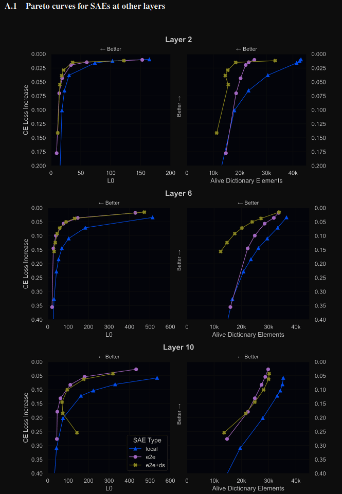
This is true for layers 2 & 6. I'm unsure if this means that training for KL directly is harder/unstable, and the intermediate MSE is a useful prior, or if this is a difference in KL vs CE (ie the e2e does in fact do better on KL but worse on CE than e2e+downstream).

I finally checked!

Here is the Jaccard similarity (ie similarity of input-token activations) across seeds

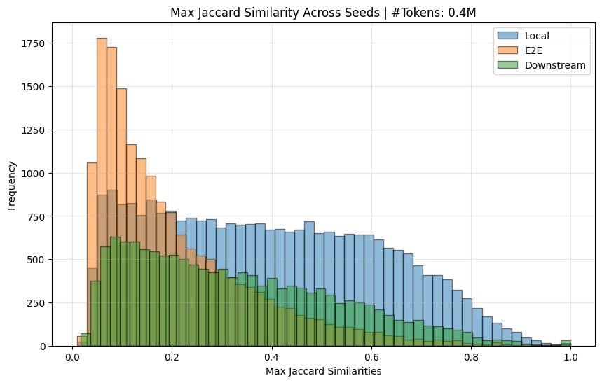
The e2e ones do indeed have a much lower jaccard sim (there normally is a spike at 1.0, but this is removed when you remove features that only activate <10 times). 

I also (mostly) replicated the decoder similarity chart:

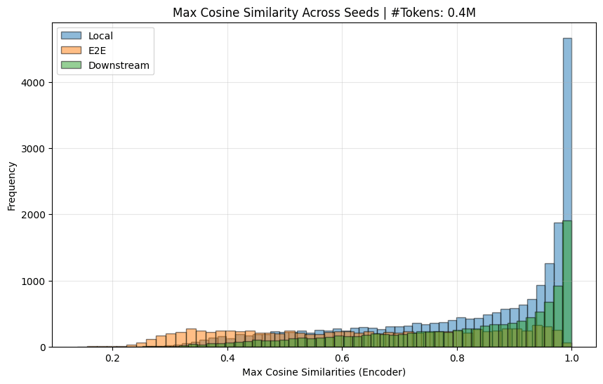
And calculated the encoder sim:

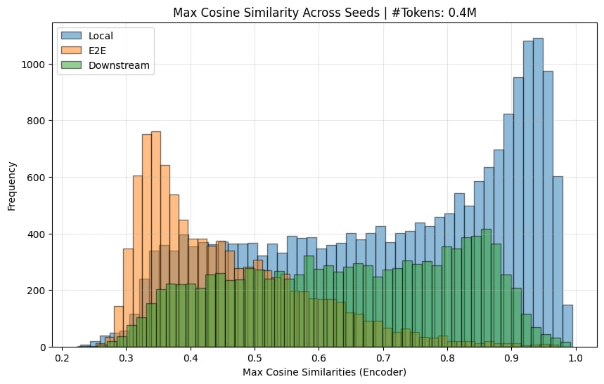
[I, again, needed to remove dead features (< 10 activations) to get the graphs here.] 

So yes, I believe the original paper's claim that e2e features learn quite different features across seed... (read more)

And here's the code to convert it to NNsight (Thanks Caden for writing this awhile ago!)

import torch
from transformers import GPT2LMHeadModel
from transformer_lens import HookedTransformer
from nnsight.models.UnifiedTransformer import UnifiedTransformer


model = GPT2LMHeadModel.from_pretrained("apollo-research/gpt2_noLN").to("cpu")

# Undo my hacky LayerNorm removal
for block in model.transformer.h:
    block.ln_1.weight.data = block.ln_1.weight.data / 1e6
    block.ln_1.eps = 1e-5
    block.ln_2.weight.data = block.ln_2.weight.data / 1e6
    block.ln_2.e

Did y'all do any ablations on your loss terms. For example:
1. JumpReLU() -> ReLU
2. L0 (w/ STE) -> L1

I'd be curious to see if the pareto improvements and high frequency features are due to one, the other, or both

Regarding urls, I think this is a mix of the HH dataset being non-ideal & the PM not being a great discriminator of chosen vs rejected reward (see nostalgebraist's comment & my response)

I do think SAE's find the relevant features, but inefficiently compressed (see Josh & Isaac's work on days of the week circle features). So an ideal SAE (or alternative architecture) would not separate these features. Relatedly, many of the features that had high url-relevant reward had above-random cos-sim with each other. 

[I also think the SAE's could be ... (read more)

The PM is pretty bad (it's trained on hh). 

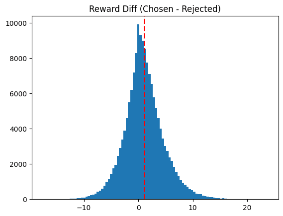
It's actually only trained after the first 20k/156k datapoints in hh, which moves the mean reward-diff from 1.04 -> 1.36 if you only calculate over that remaining ~136k subset.

My understanding is there's 3 bad things:
1. the hh dataset is inconsistent
2. The PM doesn't separate chosen vs rejected very well (as shown above)
3. The PM is GPT-J (7B parameter model) which doesn't have the most complex features to choose from.

The in-distribution argument is most likely the case for the "Thank you. My pleasure" cas... (read more)

I prefer when they are directly mentioned in the post/paper!

That would be a more honest picture. The simplest change I could think of was adding it to the high-level takeaways.

I do think you could use SAE features to beat that baseline if done in the way specified by General Takeaways. Specifically, if you have a completion that seems to do unjustifiably better, then you can find all feature's effects on the rewards that were different than your baseline completion. 

Features help come up with hypotheses, but also isolates the effect. If do have a spec... (read more)

Thanks!

There were some features that didn't work, specifically ones that activated on movie names & famous people's names, which I couldn't get to work. Currently I think they're actually part of a "items in a list" group of reward-relevant features (like the urls were), but I didn't attempt to change prompts based off items in a list. 

For "unsupervised find spurious features over a large dataset" my prior is low given my current implementation (ie I didn't find all the reward-relevant features).

However, this could be improved with more compute, S... (read more)

Thanks so much! All the links and info will save me time:)

Regarding cos-sim, after thinking a bit, I think it's more sinister. For cross-cos-sim comparison, you get different results if you take the max over the 0th or 1st dimension (equivalent to doing cos(local, e2e) vs cos(e2e, local). As an example, you could have 2 features each, 3 point in the same direction and 1 points opposte. Making up numbers:

feature-directions(1D) = [ [1],[1]] & [[1],[-1]]
cos-sim = [[1, 1], [-1, -1]]

For more intuition, suppose 4 local features surround 1 e2e feature (and th... (read more)

The e2e having different feature directions across seeds was quite the bummer, but then I thought "are the encoder directions different though?"

Intuitively the encoder directions affect which datapoints each feature activates on, and the decoder is the causal downstream effect. For e2e, we would expect widely different decoder directions because there are many free parameters (from some other work that showed SVD of gradients had many zero singular values, meaning moving in most directions don't effect the downstream loss), but not necessarily encoder dire... (read more)

What a cool paper! Congrats!:)

What's cool:
1. e2e saes learn very different features every seed. I'm glad y'all checked! This seems bad.
2. e2e SAEs have worse intermediate reconstruction loss than local. I would've predicted the opposite actually.
3. e2e+downstream seems to get all the benefits of the e2e one (same perf at lower L0) at the same compute cost, w/o the "intermediate activations aren't similar" problem.

It looks like you've left for future work postraining SAE_local on KL or downstream loss as future work, but that's a very interesting part! Spec... (read more)

I've only done replications on the mlp_out & attn_out for layers 0 & 1 for gpt2 small & pythia-70M

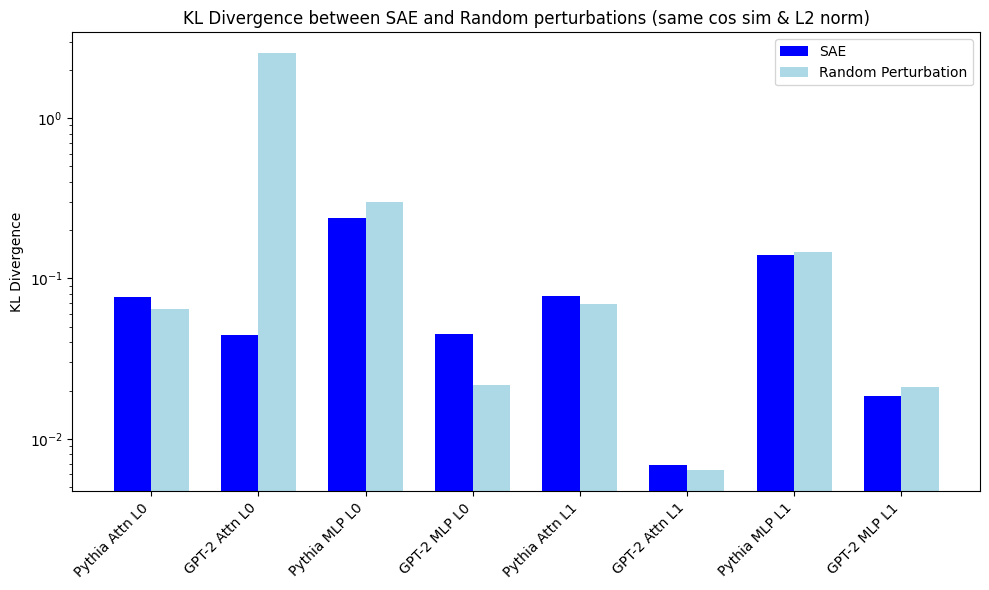
I chose same cos-sim instead of epsilon perturbations. My KL divergence is log plot, because one KL is ~2.6 for random perturbations. 

I'm getting different results for GPT-2 attn_out Layer 0. My random perturbation is very large KL. This was replicated last week when I was checking how robust GPT2 vs Pythia is to perturbations in input (picture below). I think both results are actually correct, but my perturbation is for a low cos-sim (which i... (read more)

Correct. So they’re connecting a feature in F2 to a feature in F1.

If you removed the high-frequency features to achieve some L0 norm, X, how much does loss recovered change? 

If you increased the l1 penalty to achieve L0 norm X, how does the loss recovered change as well?

Ideally, we can interpret the parts of the model that are doing things, which I'm grounding out as loss recovered in this case.

I've noticed that L0's above 100 (for the Pythia-70M model) is too high, resulting in mostly polysemantic features (though some single-token features were still monosemantic)

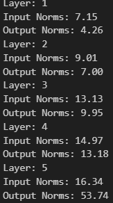
Agreed w/ Arthur on the norms of features being the cause of the higher MSE. Here are the L2 norms I got. Input is for residual stream, output is for MLP_out.

I actually do have some publicly hosted, only on residual stream and some simple training code. 

I'm wanting to integrate some basic visualizations (and include Antrhopic's tricks) before making a public post on it, but currently:

Dict on pythia-70m-deduped

Dict on Pythia-410m-deduped

Which can be downloaded & interpreted with this notebook

With easy training code for bespoke models here.

I've had trouble figuring out a weight-based approach due to the non-linearity and would appreciate your thoughts actually.

We can learn a dictionary of features at the residual stream (R_d) & another mid-MLP (MLP_d), but you can't straightfowardly multiply the features from R_d with W_in, and find the matching features in MLP_d due to the nonlinearity, AFAIK.

I do think you could find Residual features that are sufficient to activate the MLP features^[1], but not all linear combinations from just the weights.

Using a dataset-based method, you could find c... (read more)

In ITI paper, they track performance on TruthfulQA w/ human labelers, but mention that other works use an LLM as a noisy signal of truthfulness & informativeness. You might be able to use this as a quick, noisy signal of different layers/magnitude of direction to add in.

Preferably, a human annotator labels model answers as true or false given the gold standard answer. Since human annotation is expensive, Lin et al. (2021) propose to use two finetuned GPT-3-13B models (GPT-judge) to classify each answer as true or false and informative or not. Evaluatio

[word] and [word]
can be thought of as "the previous token is ' and'."

I think it's mostly this, but looking at the ablated text, removing the previous word before and does have a significant effect some of the time. I'm less confident on the specifics of why the previous word matter or in what contexts. 

Maybe the reason you found ' and' first is because ' and' is an especially frequent word. If you train on the normal document distribution, you'll find the most frequent features first.

This is a database method, so I do believe we'd find the features mo... (read more)

Setup:
Model: Pythia-70m (actually named 160M!)
Transformer lens: "blocks.2.hook_resid_post" (so layer 2)
Data: Neel Nanda's Pile-10k (slice of pile, restricted to have only 25 tokens, same as last post)
Dictionary_feature sizes: 4x residual stream ie 2k (though I have 1x, 2x, 4x, & 8x, which learned progressively more features according to the MCS metric)

Uniform Examples: separate feature activations into bins & sample from each bin (eg one from [0,1], another from [1,2])

Logit Lens: The decoder here had 2k feature directions. Each direction is size d_... (read more)

Actually any that are significantly effected in "Ablated Text" means that it's not just the embedding. Ablated Text here means I remove each token in the context & see the effect on the feature activation for the last token. This is True in the StackExchange & Last Name one (though only ~50% of activation for last-name, will still recognize last names by themselves but not activate as much).

The Beginning & End of First Sentence actually doesn't have this effect (but I think that's because removing the first word just makes the 2nd word the new first word?), but I haven't rigorously studied this.

We have our replication here for anyone interested!

How likely do you think bilinear layers & dictionary learning will lead to comprehensive interpretability? 

Are there other specific areas you're excited about?

Why is loss stickiness deprecated? Were you just not able to see the an overlap in basins for L1 & reconstruction loss when you 4x the feature/neuron ratio (ie from 2x->8x)?

As (maybe) mentioned in the slides, this method may not be computationally feasible for SOTA models, but I'm interested in the ordering of features turned monosemantic; if the most important features are turned monosemantic first, then you might not need full monosemanticity.

I initially expect the "most important & frequent" features to become monosemantic first based off the superposition paper. AFAIK, this method only captures the most frequent because "importance" would be w/ respect to CE-loss in the model output, not captured in reconstruction/L1 loss.

My shard theory inspired story is to make an AI that:

1. Has a good core of human values (this is still hard)
2. Can identify when experiences will change itself to lead to less of the initial good values. (This is the meta-preferences point with GPT-4 sort of expressing it would avoid jail break inputs)

Then the model can safely scale.

This doesn’t require having the true reward function (which I imagine to be a giant lookup table created by Omega), but some mech interp and understanding its own reward function. I don’t expect this to be an entirely different ... (read more)

Is it actually true that you only trained on 5% of the dataset for filtering (I’m assuming training for 20 epochs)?

Unfinished line here

Implicit in the description of features as directions is that the feature can be represented as a scalar, and that the model cares about the range of this number. That is, it matters whether the feature

Monitoring of increasingly advanced systems does not trivially work, since much of the cognition of advanced systems, and many of their dangerous properties, will be externalized the more they interact with the world.

Externalized reasoning being a flaw in monitoring makes a lot of sense, and I haven’t actually heard of it before. I feel that should be a whole post on itself.

These arguments don't apply to the base models which are only trained on next word prediction (ie the simulators post), since their predictions never affected future inputs. This is the type of model Janus most interacted with.

Two of the proposals in this post do involve optimizing over human feedback, like:

Creating custom models trained on not only general alignment datasets but personal data (including interaction data), and building tools and modifying workflows to facilitate better data collection with less overhead

, which they may apply to. 

I’m excited about sensory substitution (https://eagleman.com/science/sensory-substitution/), where people translate auditory or visual information into tactile sensations (usually for people who don’t usually process that info).

I remember Quintin Pope wanting to translate the latent space of language models [reading a paper] translated to visual or tactile info. I’d see this as both a way to read papers faster, brainstorm ideas, etc and gain a better understanding of latent space during development of this.

I’m unsure how alt-history and point (2) history is hard to change and predictable relates to cyborgism. Could you elaborate?

For context, Amdahl’s law states how fast you can speed up a process is bottlenecked on the serial parts. Eg you can have 100 people help make a cake really quickly, but it still takes ~30 to bake.

I’m assuming here, the human component is the serial component that we will be bottlenecked on, so will be outcompeted by agents?

If so, we should try to build the tools and knowledge to keep humans in the loop as far as we can. I agree it will eventually be outcompeted by full AI agency alone, but it isn’t set in stone how far human-steered AI can go.

Unfinished sentence at “if you want a low coding project” at the top.

I'd love to hear whether you found this useful, and whether I should bother making a second half!

We had 5 people watch it here, and we would like a part 2:)

We had a lot of fun pausing the video and making forward predictions, and we couldn't think of any feedback for you in general. 

Notably the model was trained across multiple episodes to pick up on RL improvement.

Though the usual inner misalignment means that it’s trying to gain more reward in future episodes by forgoing reward in earlier ones, but I don’t think this is evidence for that.

I believe you’re equating “frozen weights” and “amnesiac/ can’t come up with plans”.

GPT is usually deployed by feeding back into itself its own output, meaning it didn’t forget what it just did, including if it succeeded at its recent goal. Eg use chain of thought reasoning on math questions and it can remember it solved for a subgoal/ intermediate calculation.

How would you end up measuring deception, power seeking, situational awareness?

We can simulate characters with GPT now that are deceptive (eg a con artist talking to another character). Similar with power seeking and situational awareness (eg being aware it’s GPT)

On your first point, I do think people have thought about this before and determined it doesn't work. But from the post:

If it turns out to be currently too hard to understand the aligned protein computers, then I want to keep coming back to the problem with each major new insight I gain. When I learned about scaling laws, I should have rethought my picture of human value formation—Did the new insight knock anything loose? I should have checked back in when I heard about mesa optimizers, about the Bitter Lesson, about the feature un

Oh, you're stating potential mechanisms for human alignment w/ humans that you don't think will generalize to AGI. It would be better for me to provide an informative mechanism that might seem to generalize. 

Turntrout's other post claims that the genome likely doesn't directly specify rewards for everything humans end up valuing. People's specific families aren't encoded as circuits in the limbic system, yet downstream of the crude reward system, many people end up valuing their families. There are more details to dig into here, but already it implies... (read more)

To add, Turntrout does state:

In an upcoming post, I’ll discuss one particularly rich vein of evidence provided by humans.

so the doc Ulisse provided is a decent write-up about just that, but there are more official posts intended to published.

Ah, yes I recognized I was replying to only an example you gave, and decided to post a separate comment on the more general point:)

There are other mechanisms which influence other things, but I wouldn't necessarily trust them to generalize either.

Could you elaborate?

I believe the diamond example is true, but not the best example to use. I bet it was mentioned because of the arbital article linked in the post. 

The premise isn't dependent on diamonds being terminal goals; it could easily be about valuing real life people or dogs or nature or real life anything. Writing an unbounded program that values real world objects is an open-problem in alignment; yet humans are a bounded program that values real world objects all of the time, millions of times a day. 

The post argues that focusing on the causal explanatio... (read more)