Agenty things have the type signature (A -> B) -> A. In English: agenty things have some model (A -> B) which predicts the results (B) of their own actions (A). They use that model to decide what actions to perform: (A -> B) -> A.

In the context of causal DAGs, the model (A -> B) would itself be a causal DAG model $M$ - i.e. some Python code defining the DAG. Logically, we can represent it as:

$M=“\left(P\right[A|M]=f_A(A\left)\right)\&\left(P\right[B|A,M]=f_B(B,A\left)\right)”$

… for some given distribution functions $f_A$ and $f_B$.

From an outside view, the model (A -> B) causes the choice of action A. Diagrammatically, that looks something like this:

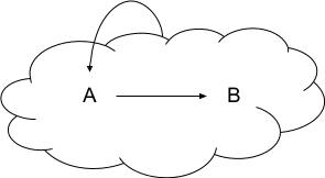
The “cloud” in this diagram has a precise meaning: it’s the model $M$ for the DAG inside the cloud.

Note that this model does not contain any true loops - there is no loop of arrows. There’s just the Hofstaderian “strange loop”, in which node A depends on the model of later nodes, rather than on the later nodes themselves.

How would we explicitly write this model as a Bayes net?

The usual way of writing a Bayes net is something like:

$P\left[X\right]={\prod }_{i}P\left[X_i|X_{pa\left(i\right)}\right]$

… but as discussed in the previous post, there’s really an implicit model M in there. Writing everything out in full, a typical Bayes net would be:

$P\left[X|M\right]={\prod }_{i}P[X_i|X_{pa\left(i\right)},M]$

… with $M=“{\forall }_i:P[X_i|X_{pa\left(i\right)},M]=f_i(X_i,X_{pa\left(i\right)})”$.

Now for the interesting part: what happens if one of the nodes is agenty, i.e. it performs some computation directly on the model? Well, calling the agenty node A, that would just be a term $P\left[A|M\right]$... which looks exactly like a plain old root node. The model M is implicitly an input to all nodes anyway, since it determines what computation each node performs. But surely our strange loop is not the same as the simple model A -> B? What are we missing? How does the agenty node use $M$ differently from other nodes?

What predictions would (A -> B) -> A make which differ from A -> B?

Answer: interventions/counterfactuals.

Modifying M

If A is determined by a computation on the model $M$, then $M$ is causally upstream of A. That means that, if we change $M$ - e.g. by an intervention $M\leftarrow do(B=2,M)$ - then A should change accordingly.

Let’s look at a concrete example.

We’ll stick with our (A -> B) -> A system. Let’s say that A is an investment - our agent can invest anywhere from $0 to $1. B is the payout of the investment (which of course depends on the investment amount). The “inner” model $M=“P[B|A,M]=f_B(B,A)”$ describes how B depends on A.

We want to compare two different models within this setup:

• A chosen to maximize some expected function of net gains, based on $M$
• A is just a plain old root node with some value (which just so happens to maximize expected net gains for the $M$ we're using)

What predictions would the two make differently?

Well, the main difference is what happens if we change the model $M$, e.g. by intervening on B. If we intervene on B - i.e. fix the payout at some particular value - then the “plain old root node” model predicts that investment A will stay the same. But the strange loop model predicts that A will change - after all, the payout no longer depends on the investment, so our agent can just choose not to invest at all and still get the same payout.

In game-theoretic terms: agenty models and non-agenty models differ only in predictions about off-equilibrium (a.k.a. interventional/counterfactual) behavior.

Practically speaking, the cleanest way to represent this is not as a Bayes net, but as a set of structural equations. Then we’d have:

$M=“P[U_i=u|M]=I[0\le u<1]duA=f_A(M,U_A)B=f_B(A,U_B)”$

However, this makes the key point a bit tougher to see: the main feature which makes the system “agenty” is that M appears explicitly as an argument to a function, not just as prior information in probability expressions.