Thanks a lot for writing up this post! This felt much clearer and more compelling to me than the earlier versions I'd heard, and I broadly buy that this is a lot of what was going on with the phase transitions in my grokking work.
The algebra in the rank-1 learning section was pretty dense and not how I would have phrased it, so here's my attempt to put it in my own language:
We want to fit to some fixed rank 1 matrix , with two learned vectors , forming . Our objective function is . Rank one matrix facts - and .
So our loss function is now . So what's the derivative with respect to x? This is the same question as "what's the best linear approximation to how does this function change when ". Here we can just directly read this off as
The second term is an exponential decay term, assuming the size of y is constant (in practice this is probably a good enough assumption). The first term is the actual signal, moving along the correct direction, but is proportional to how well the other part is doing, which starts bad and then increases, creating the self-reinforcing properties that make it initially start slow then increase.
Another rephrasing - x consists of a component in the correct direction (a), and the rest of x is irrelevant. Ditto y. The components in the correct directions reinforce each other, and all components experience exponential-ish decay, because MSE loss wants everything not actively contributing to be small. At the start, the irrelevant components are way bigger (because they're in the rank 99 orthogonal subspace to a), and they rapidly decay, while the correct component slowly grows. This is a slight decrease in loss, but mostly a plateau. Then once the irrelevant component is small and the correct component has gotten bigger, the correct signal dominates. Eventually, the exponential decay is strong enough in the correct direction to balance out the incentive for future growth.
Generalising to higher dimensional subspaces, "correct and incorrect" component corresponds to the restriction to the subspace of the a terms, and to the complement of that, but so long as the subspace is low rank, "irrelevant component bigger so it initially dominates" still holds.
My remaining questions - I'd love to hear takes:
- The rank 2 case feels qualitatively different from the rank 1 case because there's now a symmetry to break - will the first component of Z match the first or second component of C? Intuitively, breaking symmetries will create another S-shaped vibe, because the signal for getting close to the midpoint is high, while the signal to favour either specific component is lower.
- What happens in a cross-entropy loss style setup, rather than MSE loss? IMO cross-entropy loss is a better analogue to real networks. Though I'm confused about the right way to model an internal sub-circuit of the model. I think the exponential decay term just isn't there?
- How does this interact with weight decay? This seems to give an intrinsic exponential decay to everything
- How does this interact with softmax? Intuitively, softmax feels "S-curve-ey"
- How does this with interact with Adam? In particular, Adam gets super messy because you can't just disentangle things
- Even worse, how does it interact with AdamW?
I agree with both of your rephrasings and I think both add useful intuition!
Regarding rank 2, I don't see any difference in behavior from rank 1 other than the "bump" in alignment that Lawrence mentioned. Here's an example:
This doesn't happen in all rank-2 cases but is relatively common. I think usually each vector grows primarily towards 1 or the other target. If two vectors grow towards the same target then you get this bump where one of them has to back off and align more towards a different target [at least that's my current understanding, see my reply to Lawrence for more detail!].
What happens in a cross-entropy loss style setup, rather than MSE loss? IMO cross-entropy loss is a better analogue to real networks. Though I'm confused about the right way to model an internal sub-circuit of the model. I think the exponential decay term just isn't there?
What does a cross-entropy setup look like here? I'm just not sure how to map this toy model onto that loss (or vice-versa).
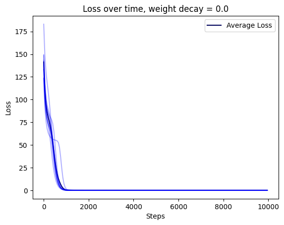
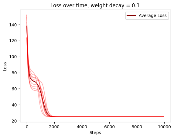
How does this interact with weight decay? This seems to give an intrinsic exponential decay to everything
Agreed! I expect weight decay to (1) make the converged solution not actually minimize the original loss (because the weight decay keeps tugging it towards lower norms) and (2) accelerate the initial decay. I don't think I expect any other changes.
How does this interact with softmax? Intuitively, softmax feels "S-curve-ey"
I'm not sure! Do you have a setup in mind?
How does this with interact with Adam? In particular, Adam gets super messy because you can't just disentangle things. Even worse, how does it interact with AdamW?
I agree this breaks my theoretical intuition. Experimentally most of the phenomenology is the same, except that the full-rank (rank 100) case regains a plateau.
Here's rank 2:
rank 10:
(maybe there's more 'bump' formation here than with SGD?)
rank 100:
It kind of looks like the plateau has returned! And this replicates across every rank 100 example I tried, e.g.
The plateau corresponds to a period with a lot of bump formation. If bumps really are a sign of vectors competing to represent different chunks of subspace then maybe this says that Adam produces more such competition (maybe by making different vectors learn at more similar rates?).
I'd be curious if you have any intuition about this!
The plateau corresponds to a period with a lot of bump formation. If bumps really are a sign of vectors competing to represent different chunks of subspace then maybe this says that Adam produces more such competition (maybe by making different vectors learn at more similar rates?).
I caution against over-interpreting the results of single runs -- I think there's a good chance the number of bumps varies significantly by random seed.
What happens in a cross-entropy loss style setup, rather than MSE loss? IMO cross-entropy loss is a better analogue to real networks. Though I'm confused about the right way to model an internal sub-circuit of the model. I think the exponential decay term just isn't there?
There's lots of ways to do this, but the obvious way is to flatten C and Z and treat them as logits.
Something like this?
def loss(learned, target):
p_target = torch.exp(target)
p_target = p_target / torch.sum(p_target)
p_learned = torch.exp(learned)
p_learned = p_learned / torch.sum(p_learned)
return -torch.sum(p_target * torch.log(p_learned))
Well, I'd keep everything in log space and do the whole thing with log_sum_exp for numerical stability, but yeah.
EDIT: e.g. something like:
import torch.nn.functional as F
def cross_entropy_loss(Z, C):
return -torch.sum(F.log_softmax(Z) * C)
C needs to be probabilities, yeah. Z can be any vector of numbers. (You can convert C into probabilities with softmax)
So indeed with cross-entropy loss I see two plateaus! Here's rank 2:
(note that I've offset the loss to so that equality of Z and C is zero loss)
I have trouble getting rank 10 to find the zero-loss solution:
But the phenomenology at full rank is unchanged:
(Adam Jermyn ninja'ed my rank 2 results as I forgot to refresh, lol)
Weight decay just means the gradient becomes , which effectively "extends" the exponential phase. It's pretty easy to confirm that this is the case:
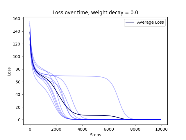
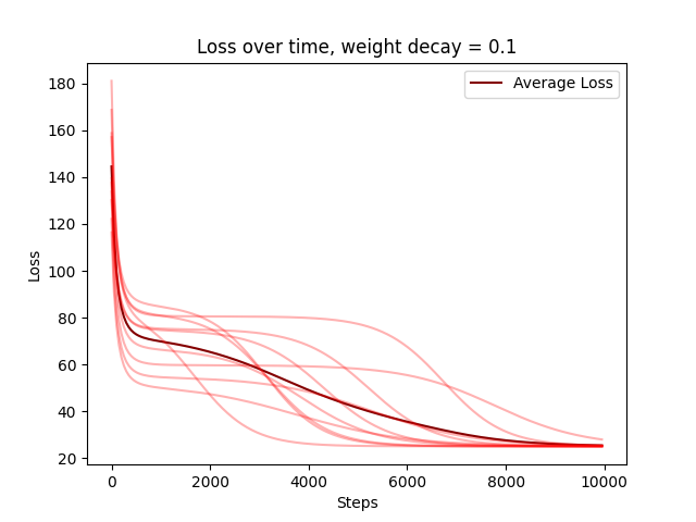
You can see the other figures from the main post here:
https://imgchest.com/p/9p4nl6vb7nq
(Lighter color shows loss curve for each of 10 random seeds.)
Here's my code for the weight decay experiments if anyone wants to play with them or check that I didn't mess something up: https://gist.github.com/Chanlaw/e8c286629e0626f723a20cef027665d1
How does this with interact with Adam? In particular, Adam gets super messy because you can't just disentangle things. Even worse, how does it interact with AdamW?
Should be trivial to modify my code to use AdamW, just replace SGD with Adam on line 33.
EDIT: ran the experiments for rank 1, they seem a bit different than Adam Jermyn's results - it looks like AdamW just accelerates things?
This is a really cool toy model, and also is consistent with Neel Nanda's Modular Addition grokking work.
Do you know what's up with the bump on the Inner Product w/Truth figures? The same bumps occur consistently for many metrics on several toy tasks, including in the Modular Addition grokking work.
EDIT: if anyone wants to play with the results in this paper, here's a gist I whipped up:
https://gist.github.com/Chanlaw/e8c286629e0626f723a20cef027665d1
I don't, but here's my best guess: there's a sense in which there's competition among vectors for which learned vectors capture which parts of the target span.
As a toy example, suppose there are two vectors, and , such that the closest target vector to each of these at initialization is . Then both vectors might grow towards . At some point is represented enough in the span, and it's not optimal for two vectors to both play the role of representing , so it becomes optimal for at least one of them to shift to cover other target vectors more.
For example, from a rank-4 case with a bump, here's the inner product with a single target vector of two learned vectors:
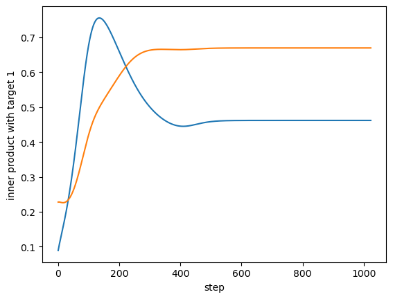
So both vectors grow towards a single target, and the blue one starts realigning towards a different target as the orange one catches up.
Two more weak pieces of evidence in favor of this story:
- We only ever see this bump when the rank is greater than 1.
- From visual inspection, bumps are more likely to peak at higher levels of alignment than lower levels, and don't happen at all in initial norm-decay phase, suggesting the bump is associated with vectors growing (rather than decaying).
Oh, huh, that makes a lot of sense! I'll see if I can reproduce these results.
For example, from a rank-4 case with a bump, here's the inner product with a single target vector of two learned vectors.
I'm not sure this explains the grokking bumps from the mod add stuff -- I'm not sure what the should be "competition" should be given we see the bumps on every key frequency.
(Thanks to Oliver Balfour, Ben Toner, and various MLAB participants for early investigations into S-curves. Thanks to Nate Thomas and Evan Hubinger for helpful comments.)
Introduction
Some machine learning tasks depend on just one component in a model. By this we mean that there is a single parameter or vector inside a model which determines the model’s performance on a task. An example of this is learning a scalar using gradient descent, which we might model with the loss function
L=12(a−~a)2Here a is the target scalar and ~a is our model of that scalar. Because the loss gradients are linear gradient descent converges exponentially quickly, as we see below:
The same holds for learning a vector using gradient descent with the loss
L=12∑i(ai−~ai)2because the loss is a sum of several terms, each of which only depends on a single component.
By contrast, some tasks depend on multiple components simultaneously. That is, the model will only perform well if multiple different parameters are near their optimal values simultaneously. Attention heads area a good example here: they only perform well if the key, query, value, and output matrices are all close to some target. If any of these are far off the whole structure fails to perform.
We think that such multi-component tasks are behind at least some occurrences of the commonly-seen S-curve motif, where the loss plateaus for an extended period before suddenly dropping. Below we provide toy examples of multi-component tasks, reason through why their losses exhibit S-curves, and explore how the structures of these S-curves vary with the ranks of the components involved. We additionally provide evidence for our explanations from numerical experiments.
Examples
Rank-1 learning
Suppose we’re using gradient descent on the regression task:
Aij=aibj~Aij=~ai~bjL=12∑ij(Aij−~Aij)2Here there is a target matrix A which has rank 1, and which we model by an outer product of two vectors ~a and ~b.
The loss gradients are:
−∂L∂ai=a(b⋅~b)−~a~b2−∂L∂bj=b(a⋅~a)−~b~a2If we write
∂~ai∂t=−∂L∂~aiand likewise for ~b we get a non-linear ordinary differential equation (ODE) of the form
d~adt=a(b⋅~b)−~a~b2d~bdt=b(a⋅~a)−~b~a2If the vectors are high-dimensional and we choose a random initialization then we approximately have a⊥~a and b⊥~b at early times. This means the above equations are, to first order,
d~adt=−~b2~ad~bdt=−~a2~bThe equation for ~a is linear in ~a, and likewise for ~b, so the initial solution decays (approximately) exponentially, which decreases the loss. At the same time, the next-order correction contains a term
d~adt=a(b⋅~b)d~bdt=b(a⋅~a)This causes the model to learn the ground truth. The true component grows linearly at first (during the exponential decay of the initialization). Then this component is actually the dominant term, so that ~a∥a and ~b∥b, and we get exponential growth of the true solution. Eventually ~a and ~b approach a and b in magnitude and the growth levels off (becomes logistic).
To summarize:
Thus, we get an exponential decay followed by a sigmoid.
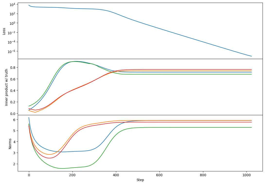
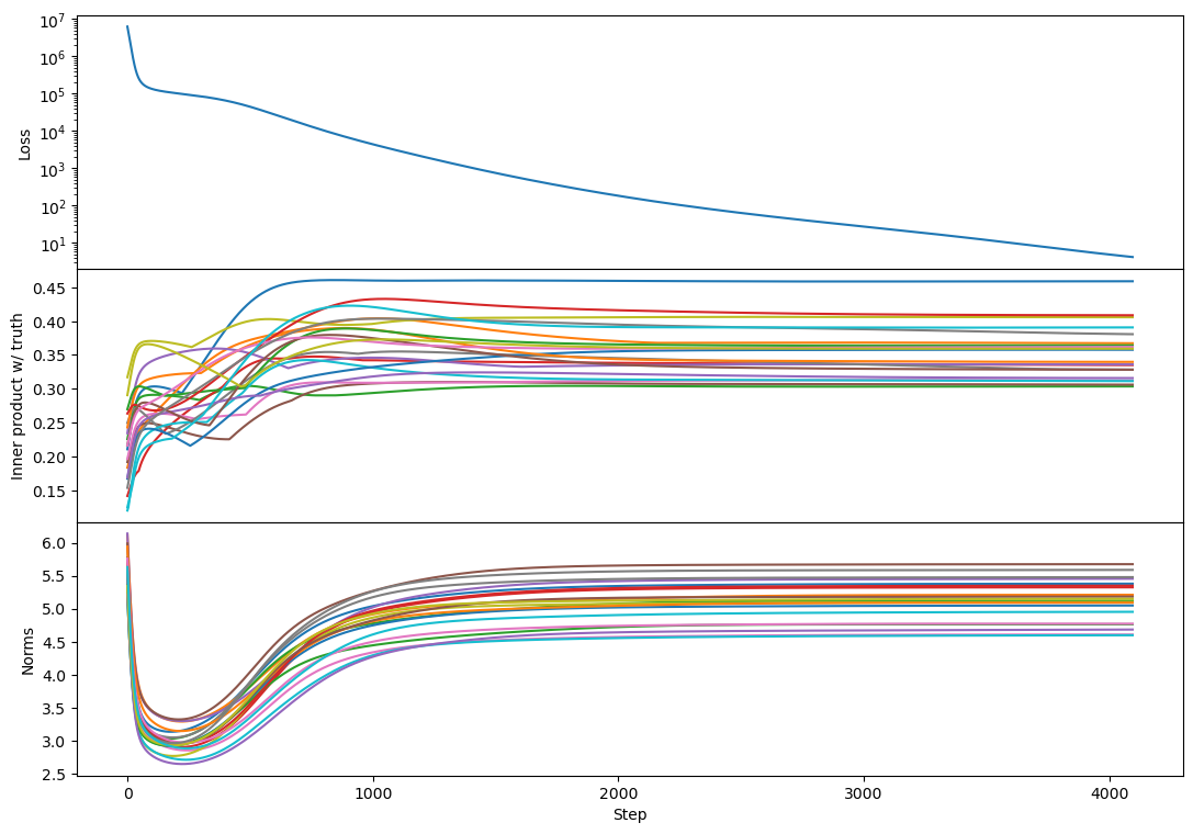
We again confirm this experimentally:
Initially the vectors just decay, giving exponential loss improvement, then the growing part takes over, bringing them into alignment with ground truth and raising their norms, resulting in a second exponential and hence an S-curve.
Low-rank learning
Similar reasoning applies to the case of learning a low-rank matrix with a low-rank representation of that matrix. Concretely, our task is now:
Aij=∑kakibkj~Aij=∑k~aki~bkjL=12∑ij(Aij−~Aij)2The loss gradients are:
−∂L∂aki=(A−~A)⋅~bk−∂L∂bkj=~ak⋅(A−~A)Notice that the resulting ODE is segmented k-by-k.
If we write
∂~ai∂t=−∂L∂~aiand likewise for ~b we get a non-linear ODE of the form
d~akdt=(A−~A)⋅~bkd~bkdt=(A−~A)T⋅~akOnce more if the vectors are high-dimensional and we choose a random initialization then we approximately have a⊥~a and b⊥~b at early times. We also have ~aj⊥~ak∀j≠k and likewise for ~bk. This means the above equations are, to first order,
d~akdt=−~bk2~akd~bkdt=−~ak2~bkso the initial solution decays (approximately) exponentially, which decreases the loss. At the same time, the next-order correction contains a term
d~akdt=ak(bk⋅~bk)d~bkdt=bk(ak⋅~ak)This causes the model to learn the truth. The true component grows linearly at first (during the exponential decay of the initialization). Then this component is actually the dominant term, ~a∥′a,~b∥b and we get exponential growth with rate |a||b|.
Eventually ~a and ~b approach a and b in magnitude and the growth levels off (becomes logistic).
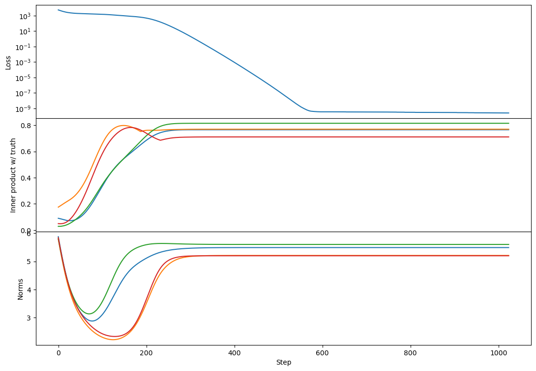
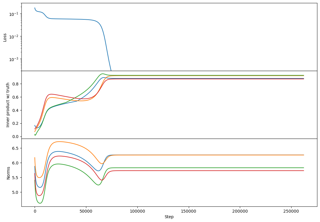
This results in the same phenomenology as in the rank-1 case, and that’s indeed what we see:
High-rank learning
(Edit: Due to a plotting bug the inner product panels in this section were not correctly normalized. I've corrected the plots below, though nothing qualitative changes.)
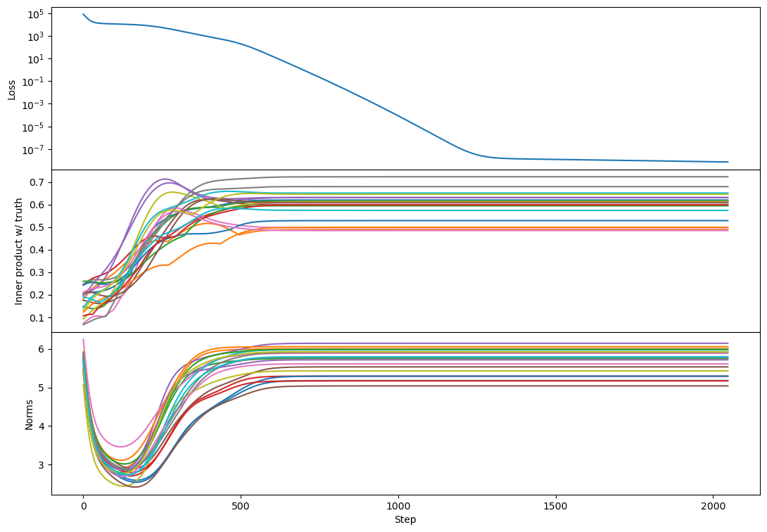
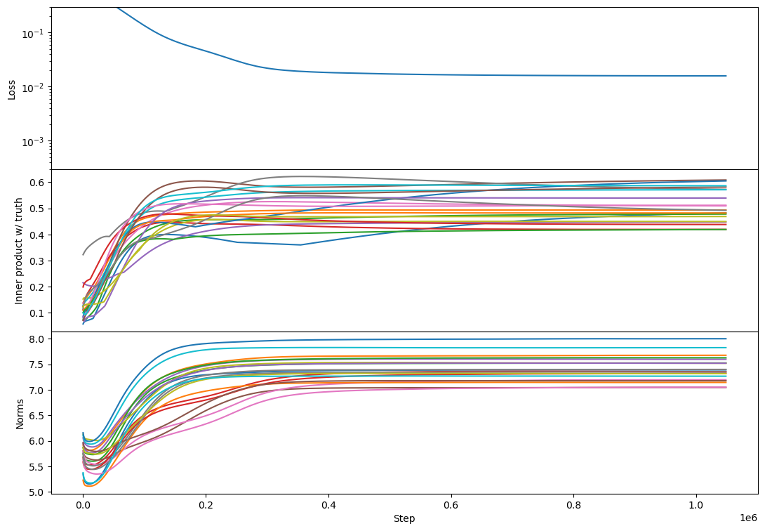
The phenomenology changes as we increase the rank. Working with 100-dimensional vectors, we see that rank-10 matrices have a similar phenomenology but with a more extended plateau:
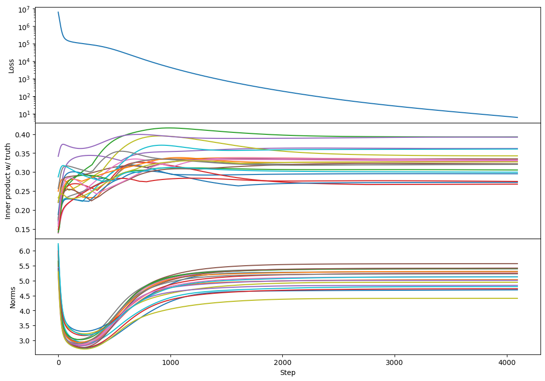
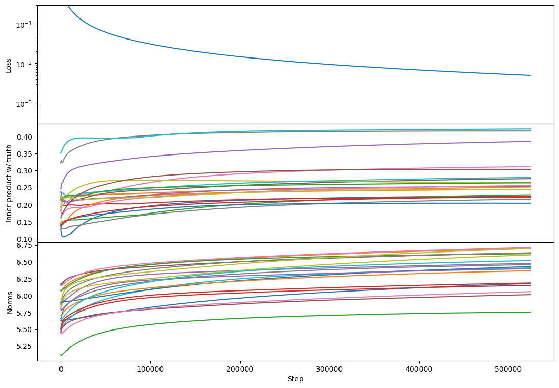
Rank-100 (full-rank) shows no second phase of exponential decay! It just transitions from exponential at the start (as norms decay) into a power-law:
(Just showing a few vectors.)
Note that the final vectors are not parallel to the ground truth: this is possible because there are many vectors, so they just need to find directions that allow them to span the same vector space as the ground truth.
To make sense of this change we start with the same ODE as before, but write it with ~a,~b as matrices whose second index runs through the different vectors:
d~adt=(A−~A)⋅~b=(a⋅bT−~a⋅~bT)⋅~b=a⋅(bT⋅~b)−~a⋅(~bT⋅~b)d~bdt=(A−~A)T⋅~a=(b⋅aT−~b⋅~aT)⋅~a=b⋅(aT⋅~a)−~b⋅(~aT⋅~a)Now comes the fun part: QT⋅Q is a positive semi-definite matrix so long as Q is real (which we’ll assume applies to our matrices). That means that the second term in each equation causes decay (which is exponential if the other of ~a,~b is held constant). For example, if we ignore the first term in the first equation we have
d~adt=−~a⋅(~bT⋅~b)So long as the dual vectors of ~a lie in the span of the dual vectors of ~b we can decompose ~a into a sum of the right-eigenvectors of ~b (the eigenvectors that live in the dual space). The projection onto each eigenvector decays independently, and so we find exponential decay (ignoring the evolution of ~b).
If the dual vectors of ~a don’t lie in the span of the dual vectors of ~b then there will be components of ~a which do not decay. As the rank of the target matrix increases the fraction of ~a outside of the span of ~b falls, making the decay more purely exponential. This explains why we see more exponential decay in the rank-100 case than the rank-10 case.
At the same time, we also have a term a⋅(bT⋅~b), which causes a growing component in ~a proportional to the truth. This component grows in size until it comes to dominate, at which point we see both the vector norms rebound and simultaneously they come into better alignment with the target vectors. Due to the non-uniqueness of matrix decompositions they do not come into as obvious an alignment as before, but we do generally see inner products increase during this phase.
As the rank increases the initial plateau for each target vector shortens because random initial vectors are closer to aligning with the ground truth. Moreover, because different vectors are learned at different rates, increasing the rank smears the transition out. The net result is that as the rank increases towards full the S-curve loses its plateau and the exponential tail turns into a power-law.
Attention Head
As one last example, consider learning an attention head of the form:
H=(A⋅B)⊗(C⋅D)where the inner dimensions of A,B and C,D are low-rank. To keep the setup simple, we’ll try learn this using the loss
L=||H−~H||2=||H||2+||~H||2−2Tr[H⋅~H]Note that this drops the softmax and is a totally artificial loss function. Nonetheless, it has the property that the loss is only low if all four components of the attention head are close to their target matrices.
The first term is irrelevant for the learning dynamics, so we drop that. The other terms we expand, finding
L=Tr[(~A⋅~B)2]Tr[(~C⋅~D)2]−2Tr[(A⋅B)⋅(~BT⋅~AT)]Tr[(C⋅D)⋅(~DT⋅~CT)]The indexing on this gets tricky, so let’s make that explicit:
L=~Aij~Bjk~BTkl~ATli~Cmn~Dno~DTop~CTpm−2AijBjk~BTkl~ATliCmnDno~DTop~CTpmTaking the gradients with respect to our parameters we find:
∂L∂~Aαβ=2~Bβk~BTkl~ATlα~Cmn~Dno~DTop~CTpm−2AαjBjk~BTkβCmnDno~DTop~CTpmThe other expressions are structurally the same so we focus on just this one. Cleaning it up a bit we find
∂L∂~A=2(~A⋅~B⋅~BT)Tr[(~C⋅~D)2]−2(A⋅B⋅~BT)Tr[(C⋅D)⋅(~DT⋅~CT)]Early in training, the final trace is nearly zero because the vectors are mostly orthogonal. So we just have the first term, giving
d~Adt=−2(~A⋅~B⋅~BT)Tr[(~C⋅~D)2]What does this evolution do to the norm of ~A? Well,
d|~A|2dt=−4Tr[(~A⋅~B)2]Tr[(~C⋅~D)2]So the norm decays exponentially at early times. What happens at later times? The second term comes to dominate so
d~Adt=−2(A⋅B⋅~B)Tr[(C⋅D)⋅(~DT⋅~CT)]This looks a bit like terms we’ve seen before. In particular, B⋅BT is positive-definite, so the first factor grows a component correlated with the truth A. The trouble is that the trace factor that follows need not be positive.
So we hit a problem: the system needs to get all of the vectors close enough that the gradients have a sign pointing towards a basin, at which point we should see rapid learning.
Fortunately there are many valid basins, because we can flip the signs of any pair of vectors and leave the system unchanged, and similarly matrices can be rotated by unitary operators in the dual space and leave everything unchanged. So we probably get a basin somewhere nearby.
All of which is to say, we should expect a plateau followed by a sudden drop once the basin is found, which is exactly what we see (with rank-2):
Conclusions
S-curves are a natural outcome of trying to learn tasks where performance depends simultaneously on multiple components. The more components involved the longer the initial plateau because there are more pieces that have to be in place to achieve low loss and hence to get a strong gradient signal.
As components align, the gradient signal on the other components strengthens, and the whole process snowballs. This is why we see a sudden drop in the loss following the plateau.
When the components being learned are low-rank it takes longer to learn them. This is because random initializations are further (on average) from values that minimize the loss. Put another way, with a rank-k ground truth and a rank-k model, there are ~k chances for each learned component to randomly be near one of the targets. So as the rank falls on average each component starts further from the nearest target, and the time spent on the plateau rises.
As components approach full rank, the plateau disappears. This is because the span of the random initialization vectors approaches the span of the target vectors, so there is a significant gradient signal on each component from the beginning.
We think that this picture is consistent with the findings of Barak+2022, who show that for parity learning SGD gradually (and increasingly-rapidly) amplifies a piece of the gradient signal known as the Fourier gap. Once this component is large enough learning proceeds rapidly and the loss drops to zero.
Questions
Finally, a few questions we haven’t answered and would be keen to hear more about: