* Authors sorted alphabetically.
This is a more detailed look at our work applying causal scrubbing to an algorithmic model. The results are also summarized here.
Introduction
In earlier work (unpublished), we dissected a tiny transformer that classifies whether a string of parentheses is balanced or unbalanced.[1] We hypothesized the functions of various parts of the model and how they combine to solve the classification task. The result of this work was a qualitative explanation of how this model works, but one that made falsifiable predictions and thus qualified as an informal hypothesis. We summarize this explanation below.
We found that the high-level claims in this informal hypothesis held up well (88-93% loss recovered, see the Methodology). Some more detailed claims about how the model represents information did not hold up as well (72%), indicating there are still important pieces of the model’s behavior we have not explained. See the experiments summary section for an explanation of each hypothesis refinement.
Causal scrubbing provides a language for expressing explanations in a formal way. A formal hypothesis is an account of the information present at every part of the model, how this information is combined to produce the output, and (optionally) how this information is represented. In this work, we start by testing a simple explanation, then iterate on our hypothesis either by improving its accuracy (which features of the input are used in the model) or specificity (what parts of the model compute which features, and optionally how). This iterative process is guided by the informal hypothesis that we established in prior work.
For a given formal hypothesis, the causal scrubbing algorithm automatically determines the set of interventions to the model that would not disturb the computation specified by the hypothesis. We then apply a random selection of these interventions and compare the performance to that of the original model.
Using causal scrubbing to evaluate our hypotheses enabled us to identify gaps in our understanding, and provided trustworthy evidence about whether we filled those gaps. The concrete feedback from a quantitative correctness measure allowed us to focus on quickly developing alternative hypotheses, and finely distinguish between explanations with subtle differences.
We hope this walk-through will be useful for anyone interested in developing and evaluating hypothesized explanations of model behaviors.
Setup
Model and dataset
The model architecture is a three layer transformer with two attention heads and pre layernorm:

There is no causal mask in the attention (bidirectional attention). The model is trained to classify sequences of up to 40 parentheses. Shorter sequences are padded, and the padding tokens are masked so they cannot be attended to.
The training data set consists of 100k sequences along with labels indicating whether the sequence is balanced. An example input sequence is ()())() which is labeled unbalanced. The dataset is a mixture of randomly generated sequences and adversarial examples.[2] We prepend a [BEGIN] token at the start of each sequence, and read off the classification above this token (therefore, the parentheses start at sequence position 1).
For the experiments in this writeup we only use random, non-adversarial, inputs, on which the model is almost perfect (loss of 0.0003, accuracy 99.99%). For more details of the dataset see the appendix.
Algorithm
Our hypothesis is that the model is implementing an algorithm that is approximately as follows:
- Scan the sequence from right to left and track the nesting depth at each position. That is, the nesting depth starts at 0 and then, as we move across the sequence, increments at each
)and decrements at each(.
You can think of this as an "elevation profile" of the nesting level across the sequence, which rises or falls according to what parenthesis is encountered.
Important note: scanning from left to right and scanning from right to left are obviously equally effective. The specific model we investigated scans from right to left (likely because we read off the classification at position 0). - Check two conditions:
- The Equal Count Test (aka the count test): Is the elevation back to 0 at the left-most-parentheses? This is equivalent to checking whether there are the same number of open and close parentheses in the entire sequence.
- The Above Horizon Test (aka the horizon test): Is the elevation non-negative at every position? This is equivalent to checking whether there is at least one open parenthesis
(that has not been later closed)(cf. see the third example below).
- If either test fails, the sequence is unbalanced. If both pass, the sequence is balanced.
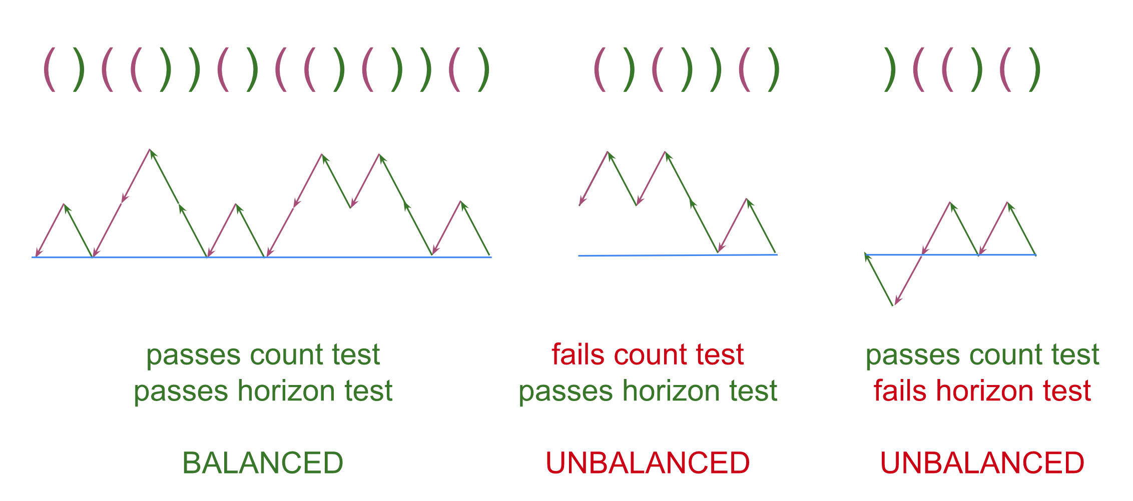
(As an aside, this is a natural algorithm; it's also similar to what codex or GPT-3 generate when prompted to balance parentheses.)
Again - this is close to the algorithm we hypothesize the model uses, but not exactly the same. The algorithm that the model implements, according to our hypothesis, has two differences from the one just described.
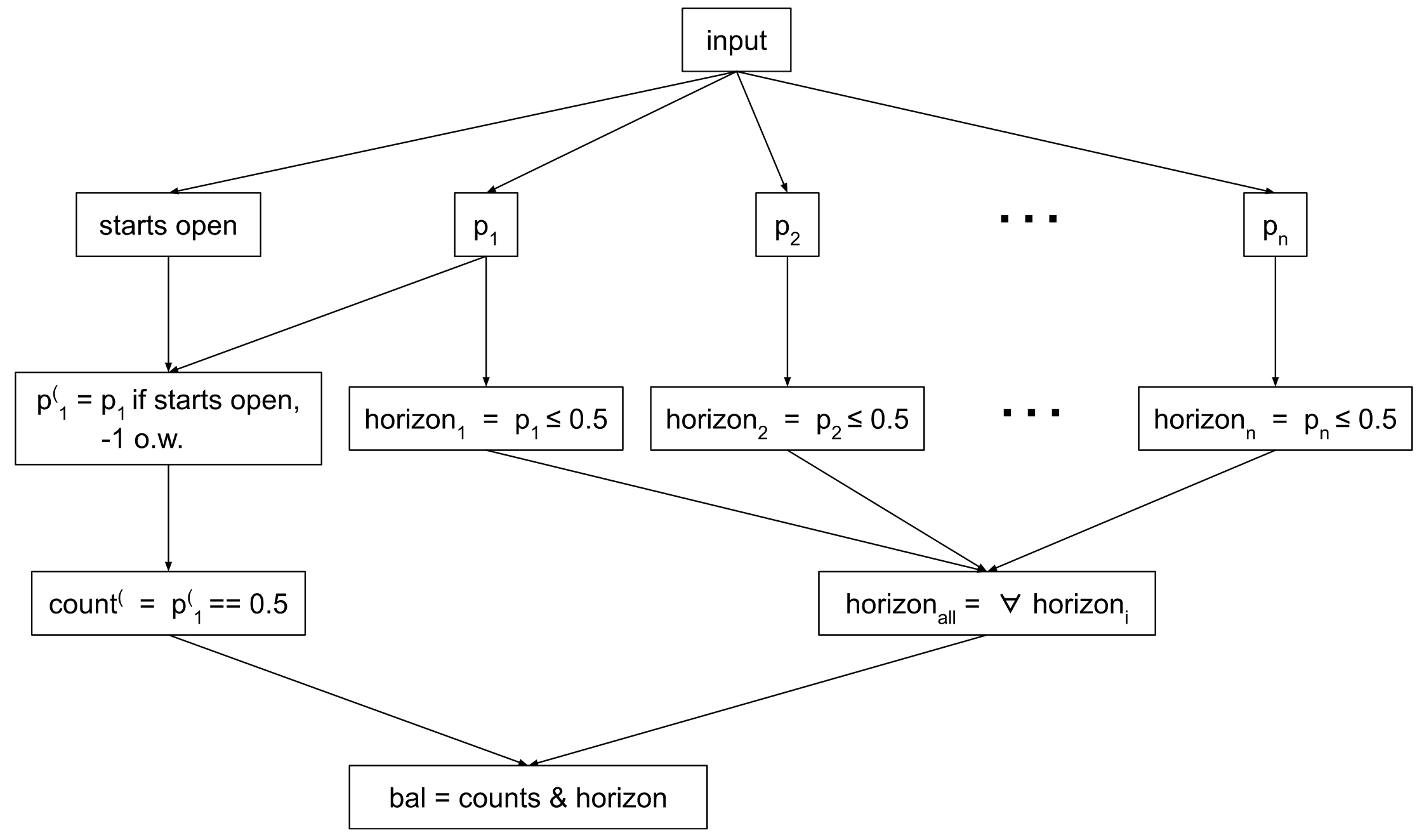
1. It uses proportions instead of ‘elevation’. Instead of computing ‘elevation’ by incrementing and decrementing a counter, we believe the model tracks the proportion of parentheses that are open in each suffix-substring (i.e. in every substring that ends with the rightmost parenthesis). This proportion contains the same information as ‘elevation’. We define:
pi: the proportion of open parentheses ( in the suffix-substring starting at position i, i.e. from i to the rightmost parenthesis
Put in terms of proportions, the Equal Count Test is whether this is exactly 0.5 for the entire string (p1 == 0.5). The Not Beneath Horizon Test is whether this is less than or equal to 0.5 for each suffix-substring (pi <= 0.5 for all i); if the proportion is less than 0.5 at any point, this test is failed.
2. It uses a combined test of, “is the first parenthesis open, and does the sequence pass Equal Count?” Call this the Start-Open-and-Equal-Count test, aka the count( Test.
Consider the Start-Open component. Sequences that start with a closed parenthesis instead of an open one cannot be balanced: they inevitably fail to meet at least one of Equal Count or Not Beneath Horizon. However, the model actually computes Start-Open separately!
As the model detects Start-Open in the circuit that computes the ‘equal count’ test, we’ve lumped them together for cleaner notation:
count(: Is the elevation back to 0 at the left-most-parenthesis (i.e. the Equal Count Test), and does the sequence start with open parenthesis? i.e. count( := (first parenthesis is open) & (passes Equal Count Test)
We can use these variables to define a computational graph that will compute if any sequence of n parentheses is balanced or not.
Note that we define count(, horizoni, and horizonall to be booleans that are true if the test passes (implying that the sequence might be balanced) and false (implying the sequence definitely isn’t balanced).
We will reference the features of the above graph to make claims about what particular components of the model compute.
Informal Hypothesis
Our prior interpretability work suggested that the model implements this algorithm in roughly the following manner:
- Head 0.0 has an upper triangular attention pattern (recall that model uses bidirectional attention): at every query position it pays roughly-equal attention to all following sequence positions and writes in opposite directions at open and close parentheses. These opposite directions are analogous to “up” and “down” in the elevation profile. Thus, head 0.0 computes every pi and writes this in a specific direction.
- The MLPs in layers 0 and 1 then transform the pi into binary features. In particular, at position 1 they compute the count( test, and at every sequence position they compute the horizon test for that position.
- Head 1.0 and 2.0 both copy the information representing the count( test from position 1 (the first parentheses token) to position 0 (the [BEGIN] token where the classifier reads from).
- Head 2.1 checks that the horizon test passed at all positions and writes this to position 0.
A consequence of this hypothesis is that at position 0, head 2.0 classifies a sequence as balanced if it passes the count( test, and classifies it as unbalanced if it fails the test. Head 2.1 does the same for the horizon test. As some evidence for this hypothesis, let’s look at an attribution experiment.
We run the model on points sampled on the random data set, which may each pass or fail either or both of the tests. We can measure the predicted influence on the logits from the output of heads 2.0 and 2.1.[3]
For each data point, we plot these two values in the x and y axes. If each head independently and perfectly performs its respective test, we should expect to see four clusters of data points:
- Those that pass both tests (i.e. are balanced) are in the top right: both heads classify them as balanced, so their x and y positions are positive.
- Unbalanced sequences, which fail both tests, are points in the bottom left.
- Sequences that pass only one of the tests should be in the top left or bottom right of the plot.
This is the actual result:
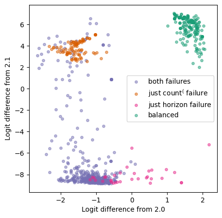
The result roughly matches what we expected, but not entirely.
The part that matches our expectations: the green (balanced) points are consistently classified as balanced by the two heads, and the orange (count( failure only) points are consistently classified as balanced by 2.1 and unbalanced by 2.0.
However, the picture for the other clusters does not match our expectations; this shows that our hypothesis is flawed or incomplete. The pink points fail only the horizon test, and should be incorrectly classified as balanced by 2.0, and correctly classified as unbalanced by 2.1. In reality, 2.0 often ‘knows’ that these sequences are unbalanced, as evidenced by about half of these points being in the negative x axis. It must therefore be doing something other than the count( test, which these sequences pass. The purple points, which fail both the count( and horizon tests, are sometimes incorrectly thought to be balanced by 2.1, so head 2.1 cannot be perfectly performing the horizon test. In Experiment 3, we’ll show that causal scrubbing can help us detect that this explanation is flawed, and then derive a more nuanced explanation of head 2.1’s behavior.
Methodology
We use the causal scrubbing algorithm in our experiments. To understand this algorithm, we advise reading the introduction post. Other posts are not necessary to understand this post, as we’ll be talking through the particular application to our experiments in detail.[4]
Following the causal scrubbing algorithm, we rewrite our model, which is a computational DAG, into a tree that does the same computation when provided with multiple copies of the input. We refer to the rewritten model as the treeified model. We perform this rewrite so we can provide separate inputs to different parts of the model–say, a reference input to the branch of the model we say is important, and a random input to the branch we say is unimportant. We’ll select sets of inputs randomly conditional on them representing the same information, according to our hypothesis (see the experiments for how we do this), run the treeified model on these inputs, and observe the loss. We call the treeified model with the separate inputs assigned according to the hypothesis the “scrubbed model”.
Before anything else, we record the loss of the model under two trivial hypotheses: “everything matters” and “nothing matters”. If a hypothesis we propose is perfect, we expect that the performance of the scrubbed model is equal to that of the baseline, unperturbed model. If the information the hypothesis specifies is unrelated to how the model works, we expect the model’s performance to go down to randomly guessing. Most hypotheses we consider are somewhere in the middle, and we express this as a % loss recovered between the two extremes. For more information on this metric, refer to the relevant section here.
Summary of experimental results
We run a series of experiments to test different formalizations of (parts of) the informal hypothesis we have about this model.
We start with a basic claim about our model: that there are only three heads whose direct contribution to the classifier head is important: 1.0 and 2.0 which compute count(, and 2.1 which computes the horizon test. We then improve this claim in two ways:
- Specificity: Making a more specific claim about how one of these pathways computes the relevant test. That is, we claim a more narrow set of features of the input are important, and therefore increase the set of allowed interventions. This is necessary if we want to claim to understand the complete computation of the model, from inputs to outputs. However, it generally increases the loss of the scrubbed model if the additions to the hypothesis are imperfect.
- Accuracy: Improving our hypothesis to more accurately match what the model computes. This often involves adjusting the features computed by our interpretation $I$. If done correctly this should decrease the loss of the scrubbed model.
A third way to iterate the hypothesis would be to make it more comprehensive, either by including paths through the model that were previously claimed to be unimportant or by being more restrictive in the swaps allowed for a particular intermediate. This should generally decrease the loss. We don’t highlight this type of improvement in the document, although it was a part of the research process as we discovered which pathways were necessary to include in our explanation.
Our experiments build upon one another in the following way:
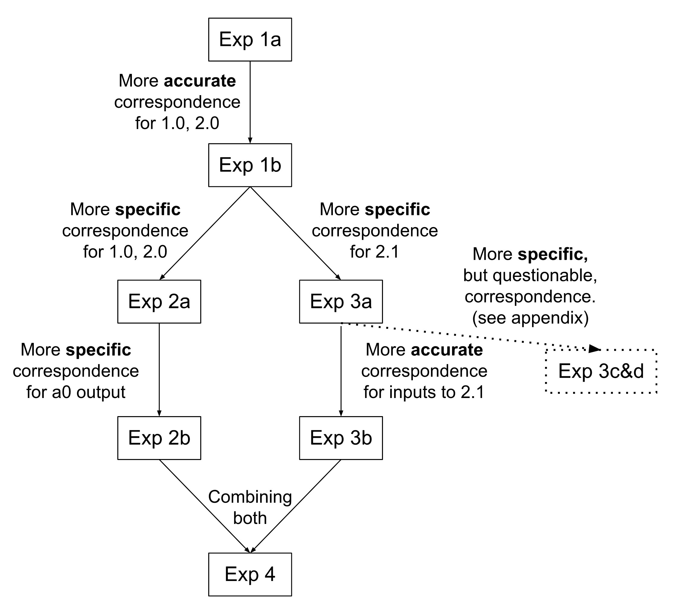
The results of the experiments are summarized in this table, which may be helpful to refer back to as we discuss the experiments individually.
| # | Summary of claimed hypothesis | Loss ± Std. Error | % loss recovered | Accuracy |
| 0a | The normal, unscrubbed, model | 0.0003 | 100% | 100% |
| 0b | Randomized baseline | 4.30 ± 0.12 | 0% | 61% |
| 1a | 1.0 and 2.0 compute the count test, 2.1 computes the horizon test, they are ANDed | 0.52 ± 0.04 | 88% | 88% |
| 1b | 1a but using the count( test | 0.30 ± 0.03 | 93% | 91% |
| 2a | More specific version of 1b, where we specify the inputs to 1.0 and 2.0 | 0.55 ± 0.04 | 88% | 87% |
| 2b | 2a but using the ɸ approximation for the output of 0.0 | 0.53 ± 0.04 | 88% | 87% |
| 3a | More specific version of 1b, where we break up the inputs to 2.1 by sequence position | 0.97 ± 0.06 | 77% | 85% |
| 3b | 3a but using padj | 0.68 ± 0.05 | 84% | 88% |
| 3c | 3a plus specifying the inputs to 2.1 at each sequence position | 0.69 ± 0.05 | 84% | 87% |
| 3d | 3a but sampling a1 at each sequence position randomly | 0.81 ± 0.05 | 81% | 87% |
| 4 | Including both 2b and 3b | 1.22 ± 0.07 | 72% | 82% |
(% loss recovered is defined to be 1 - (experiment loss - 0a loss) / 0b loss. This normalizes the loss to be between 0% and 100%, where higher numbers are better.)
All experiments are run on 2000 scrubbed inputs, sampled according to the algorithm from 100,000 sequences of parentheses.
Detailed experimental results
Experiment 0: Trivial hypothesis baseline
Running the model itself results in a loss of 0.0003 (100% accuracy) on this dataset. If you shuffle the labels randomly, this results in a loss of 4.30 (61% accuracy – recall the dataset is mostly unbalanced).
These can both be formalized as trivial hypotheses, as depicted in the diagram below. We hypothesize an interpretation with a single node, which corresponds (via ) to the entire model. The computational graph of , labeled with the model component it corresponds to, is shown below in black. The proposed feature computed by the node of I is annotated in red.
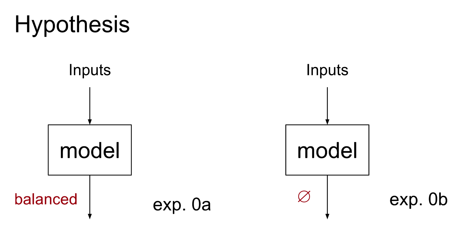
Note that in both cases we don’t split up our model into paths (aka ‘treeify’ it), meaning we will not perform any internal swaps.
In experiment 0a, we claim the output of the entire model encodes information about whether a given sequence is balanced. This means that we can swap the output of the model only if the label agrees: that is, the output on one balanced sequence for another balanced sequence. This will of course give the same loss as running the model on the dataset.
For 0b, we no longer claim any correspondence for this output. We thus swap the outputs randomly among the dataset. This is equivalent to shuffling the labels before evaluating the loss. We call such nodes (where any swap of their output is permitted) ‘unimportant’ and generally don’t include them in correspondence diagrams.
These experiments are useful baselines, and are used to calculate the % loss recovered metric.
Experiment 1: Contributions to residual stream at pos0
We claimed that the output of 1.0 and 2.0 each correspond to the count( test, and the output of 2.1 corresponds to the horizon test. Let’s check this now. In fact, we will defend a slightly more specific claim: that the direct connection[5] of these heads to the input of the final layer norm corresponds to the count( test.
1a: Testing a simple hypothesis for heads 1.0, 2.0, 2.1
To start, we’ll first test a simple hypothesis: that 1.0 and 2.0 just implement the simple Equal Count Test (notably, not the count( test) and 2.1 implements the horizon test, without checking whether the sequence starts with an open parenthesis.
We can draw this claimed hypothesis in the following diagram (for the remainder of this doc we won’t be drawing the inputs explicitly, to reduce clutter. Any node drawn as a leaf will have a single upstream input.):
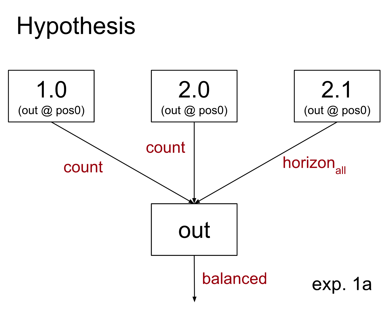
How do we apply causal scrubbing to test this hypothesis? Let’s walk through applying it for a single data point (a batch size of 1). We apply the causal scrubbing algorithm to this hypothesis and our model. This will choose 5 different input data points from the dataset described above, which we will use to run the tree-ified model on as shown below:
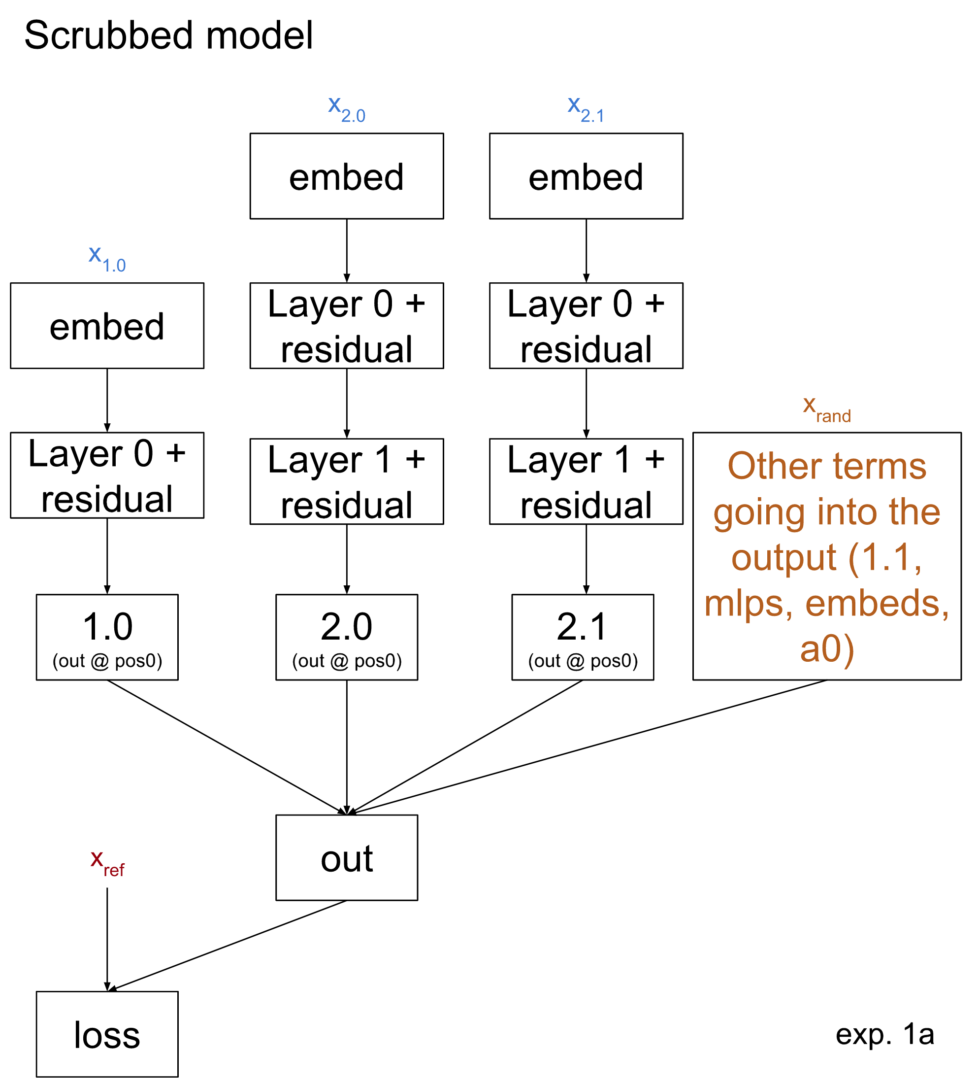
- xref, or the reference input. We compute the loss of the scrubbed model from the true label of xref. However, we will never run the scrubbed model on it; all inputs to the scrubbed model will be replaced with one of the other sampled inputs.
- Our hypothesis claims that, if we replace the output of 1.0 or of 2.0 with its output on some input x’ that agrees with xref on the count test, then the output will agree with xref on the balanced test. Therefore we sample random x1.0 and x2.0 which each agree with xref on the count test. (Note that this means x1.0 and x2.0 agree with each other on this test as well, despite being separate inputs.)
- Similarly, x2.1 is sampled randomly conditional on agreeing with xref on the horizon test.
- xrand is a random dataset example. The subtree of the model which is rooted at the output and omits the branches included in the hypothesis–that is, the branches going directly to 1.0, 2.0, and 2.1–is run on this example.
We perform the above sample-and-run process many times to calculate the overall loss. We find that the scrubbed model recovers 88% of the original loss. The scrubbed model is very biased towards predicting unbalanced, with loss of 0.25 on unbalanced samples and 1.31 on balanced samples.
1b: Additional check performed by 1.0 and 2.0: initial parenthesis open
This, however, was still testing if 1.0 and 2.0 care about only the equal count test! As described above we believe it is more accurate to say that they check the count( test, testing that the first parenthesis is open as well as performing the Equal Count Test.
Consider the set of inputs that pass the equal count test but fail the count( test.[6] Let us call these the fails-start-open set. If we return to the attribution results from the informal hypothesis we can get intuition about the model’s behavior on these inputs:
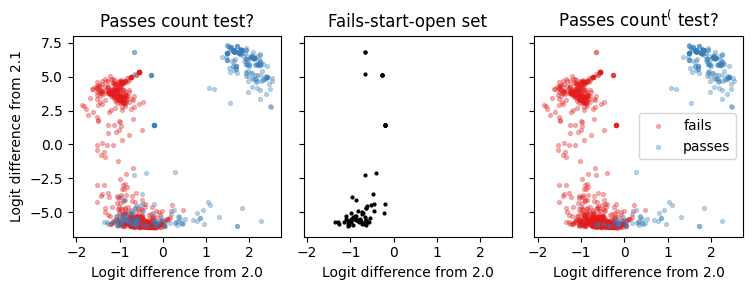
The left most figure suggests that head 2.0 is not implementing the count test, as it has a negative output on many points that pass the count test. As the center figure shows, these points correspond to points that start with ")". On the other hand, the count^( test more accurately predicts the logits of head 2.0. Taken together, these results suggest that head 2.0 is implementing the count^( test and not the count test.
The only difference from the left subfigure to the right subfigure is that the points in the fails-start-open set fail the more specific count( test. We see that indeed, the output of head 2.0 is unbalanced on these inputs. Comparing the right and left diagrams we see the count( test more cleanly predicts the output of head 2.0. The results for head 1.0 are similar.
Here is an updated hypothesis claim:
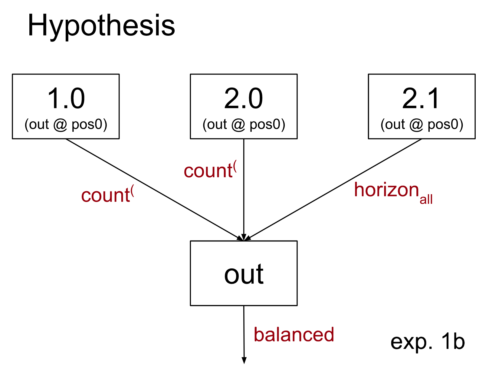
Compared to experiment 1a, the intervention is different in two ways:
- When the reference input is balanced, we may no longer sample x1.0 or x2.0 from the fails-start-open set. To the extent that our hypothesis is right and such inputs x1.0 or x2.0 cause 1.0 or 2.0 to output more “evidence of unbalance”, this change will improve our loss on balanced sequences. Eyeballing the plots above, we do expect this to happen.
- When the reference input is unbalanced, we may now sample x1.0 and x2.0 from the fails-start-open set. To the extent that our hypothesis is wrong and such inputs cause 1.0 or 2.0, respectively, to output less “evidence of unbalance”, this change will harm our loss on unbalanced sequences. Eyeballing the plots above, it is somewhat hard to tell whether we should expect this: these points do have some evidence of unbalance, but it is unclear how the magnitude compares to that of the fail-count set.
The scrubbed model recovers 93% of the loss. In particular the loss on balanced goes way down (1.31 -> 0.65) while the loss on unbalanced is slightly lower (0.25 -> 0.18). Thus this experiment supports our previous interpretability result that 1.0 and 2.0 detect whether the first parenthesis is open.
Comparing experiments 1a and 1b makes it clear the count( test is an improvement. However, it is worth noticing that if one had only the results of experiment 1a, it would not be clear that such an improvement needed to be made.[7] In general, causal scrubbing is not legibly punishing when the feature you claimed correspondance with is highly correlated with the ‘true feature’ that the component of the model is in fact picking up. We expect that all our claims, while highly correlated with the truth, will miss some nuance in the exact boundaries represented by the model.
Experiment 2: More specific explanation for 1.0’s and 2.0’s input
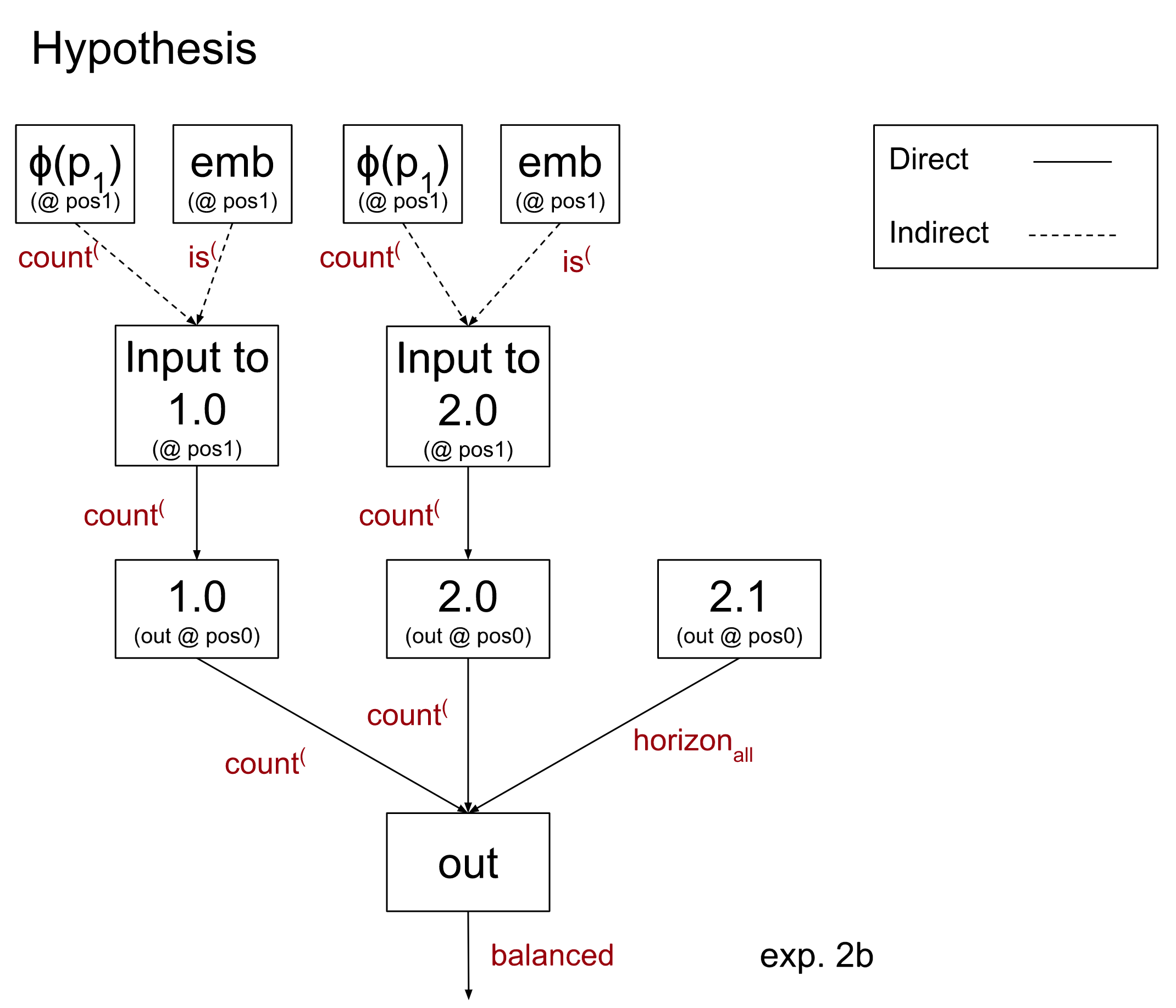
To make the above hypothesis more specific, we’ll explain how 1.0 and 2.0 compute the count( test: in particular, they use the output of 0.0 at position 1. To test this, we update the hypothesis from 1a to say that 2.0 and 1.0 only depend on whether the first parenthesis is open and whether 0.0 is run on an input that passes the count( test. The other inputs to the subtrees rooted at 1.0 and 2.0 don’t matter. We aren’t stating how the output of 0.0 and the embedding reach those later heads; we’re considering the indirect effect, i.e. via all possible paths, rather than just the direct effect that passes through no other nodes in the model.
2a: Dependency on 0.0
Our claimed hypothesis is shown below. Recall that we do not show unimportant nodes, we annotate the nodes of I with the nodes of G that they correspond to, and we annotate the edges with the feature that that node of I computes:[8]
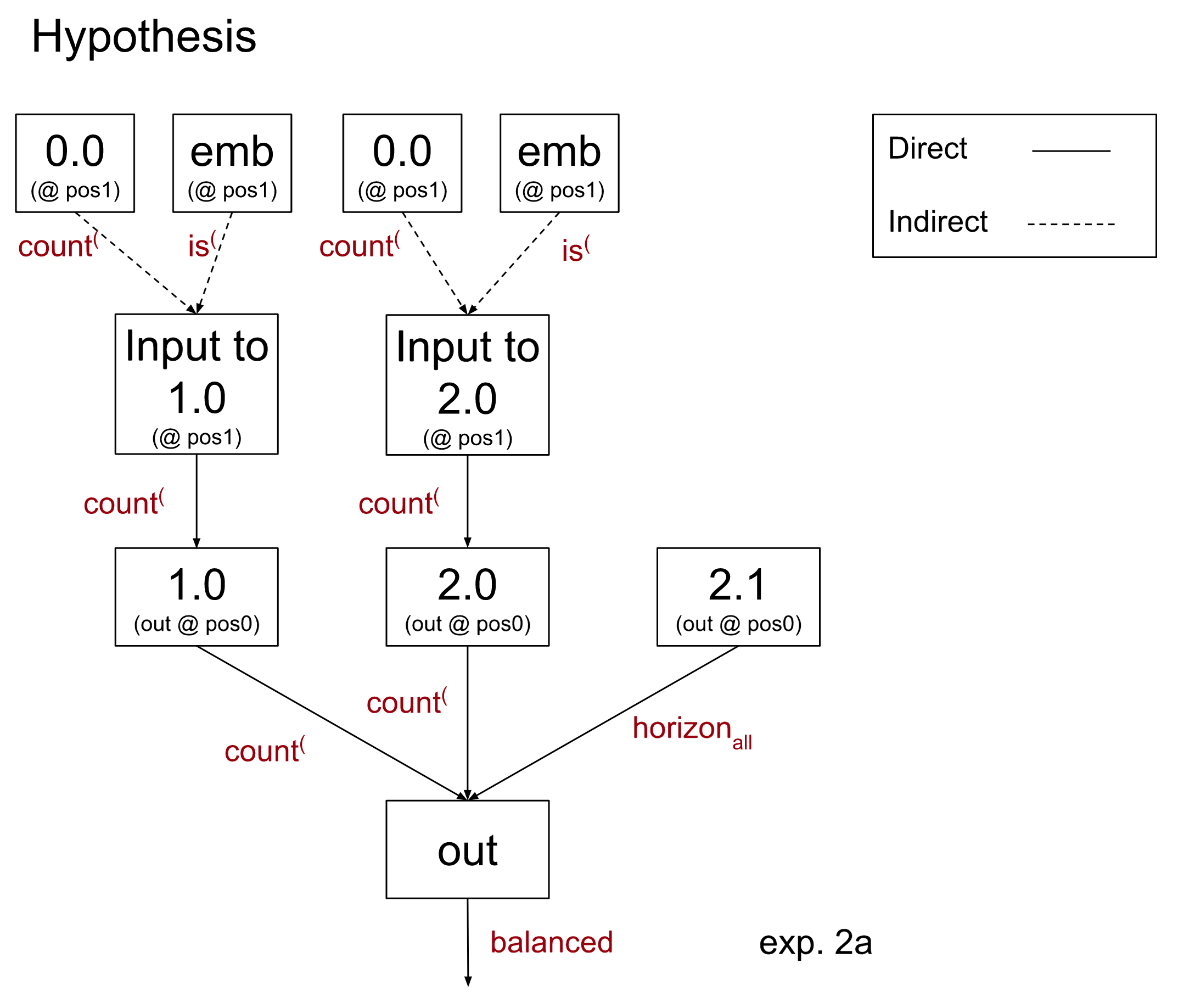
This hypothesis will result in the following treeified model:
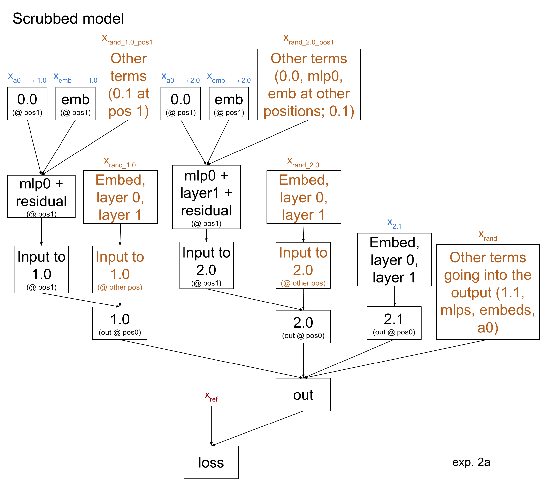
How do we determine the 5 input data points annotated in blue? Following the causal scrubbing algorithm, we first fix xref at the output. We then recursively move through the hypothesis diagram, sampling a dataset example for every node such that it agrees with the downstream nodes on the labeled features. The non-leaf node data points can then be discarded, as they are not used as inputs in the scrubbed model. This is depicted below:
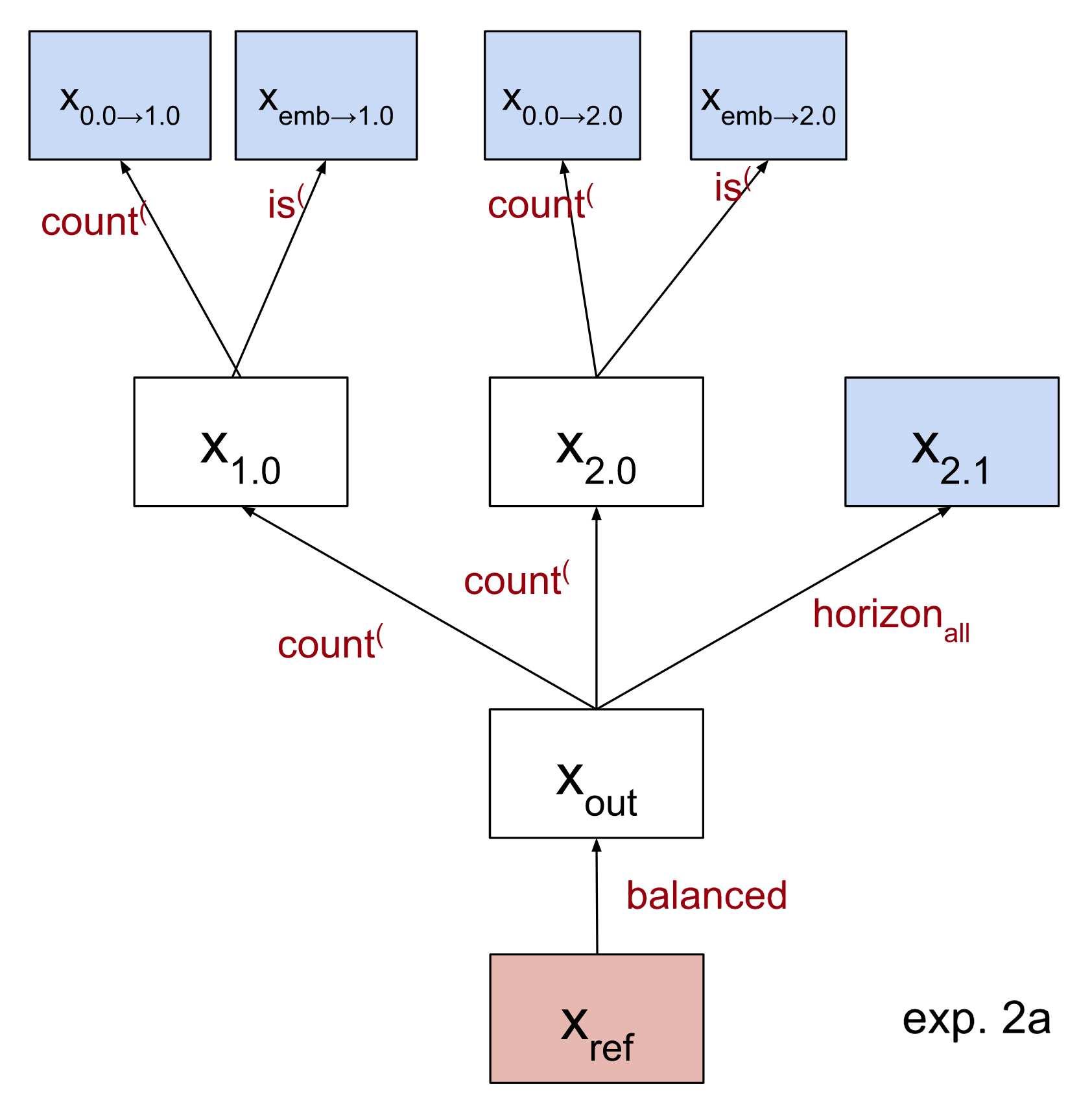
In particular, we will first choose a dataset sample xref whose label we will use to evaluate the loss of the scrubbed model. Then we will select the input datasets as follows:
- xout agrees with xref on the balanced test.
- x2.1 agrees with xref on the never beneath horizon test (as before)
- Both x1.0 and x2.0 agree with xref on the count( test.
- x0.0→1.0 agrees with x1.0 on the count( test, and similarly for 2.0.
- xemb→1.0 agrees with x1.0 on whether the sequence starts with (, and similarly for 2.0.
Note that we do not require any other agreement between inputs! For example, xemb → 1.0 could be an input that fails the count test.
The 5 inputs in orange are claimed to be unimportant by our hypothesis. This means we will sample them randomly. We do, however, use the same random value for all unimportant inputs to a particular node in our model. For instance, there are many ‘unimportant’ inputs to the final layer norm: all three mlps, attention layer 0, and head 1.1. All of these are sampled together. Meanwhile, we sample these nodes separately from unimportant inputs to other nodes (e.g. the non-position 1 inputs to head 2.0); see the appendix for some discussion of this.
The scrubbed model recovers 88% of the loss. Compared to experiment 1b, the loss recovered is significantly lower: a sign that we lost some explanatory power with this more specific hypothesis. By asserting these more specific claims, however, we still recover a large portion of the original loss. Overall, we think this result provides evidence that our hypothesis is a reasonable approximation for the 2.0 circuit. (To rule out the possibility that 0.0 is not important at all in these paths, we also ran an experiment replacing its output with that on a random input; this recovered 84% of the loss which is significantly less).
2b: 0.0’s output encodes p in a specific direction
In fact, we believe that the proportion of open parentheses is encoded linearly in a particular direction. For more details and a precise definition of how we think this is done, see the appendix. The takeaway, however, is that we have a function ɸ which maps a value of p to a predicted activation of 0.0. We can thus rewrite the output of 0.0 in our model as the sum of two terms: ɸ(p) and the residual (the error of this estimate). We then claim that the ɸ(p) term is the important one. In essence, this allows swapping around the residuals between any two inputs, while ɸ(p) can only be swapped between inputs that agree on the count( test. As a hypothesis diagram, this is:
Which leads to the following treeified model (again, with unimportant nodes in orange):
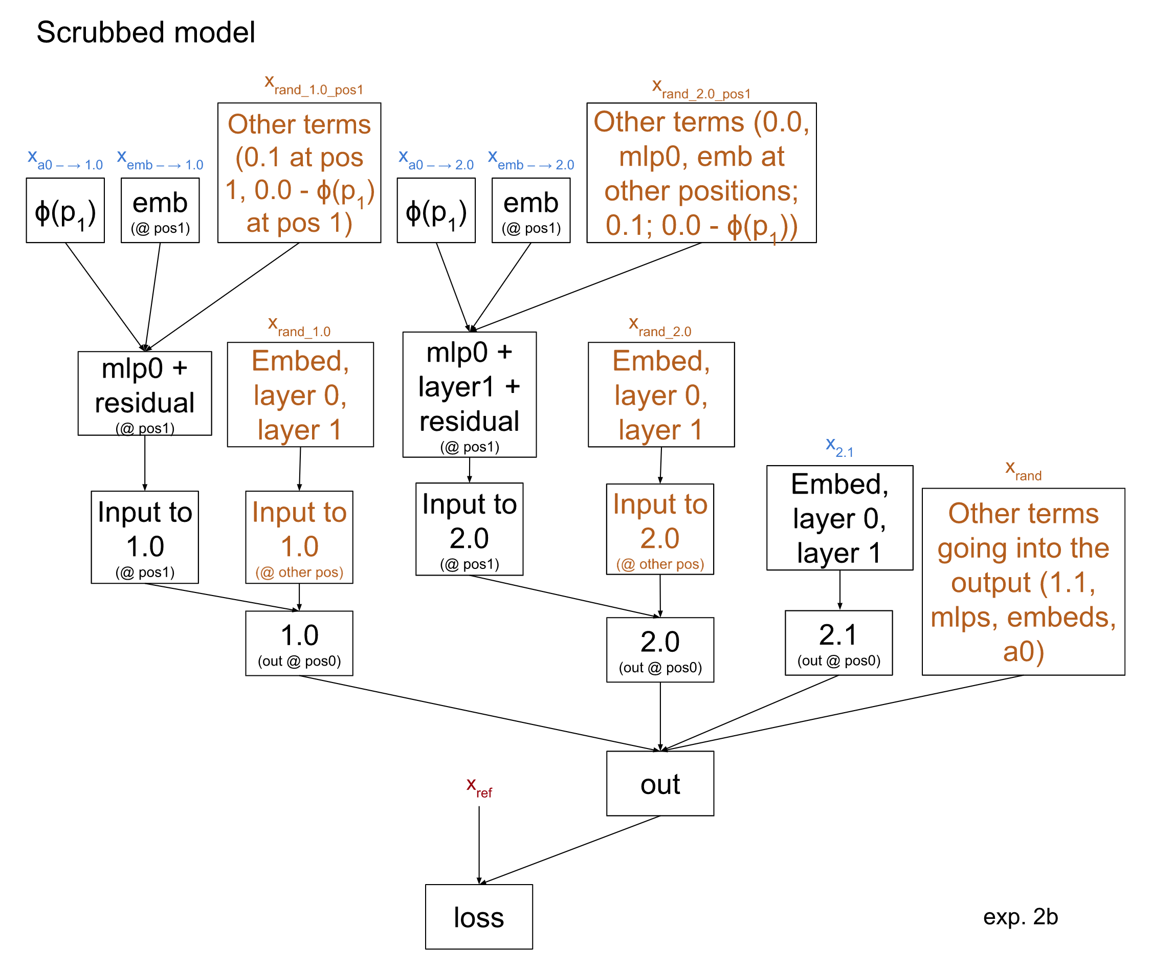
This results in a loss of 0.56, with accuracy 87%. This is basically unchanged from experiment 2a, giving evidence that we were correct in how p values are translated into the output of 0.0. Importantly, however, if we were somewhat wrong about which p values head 0.0 outputs on each input, this would have already hurt us in experiment 2a. Thus this result shouldn’t increase our confidence on that account.
Experiment 3: How does 2.1 compute the horizon condition?
For this experiment, we are not including the breakdown of 2.0 from experiment 2. We will add these back in for experiment 4, but it is simpler to consider them separately for now.
3a: Breaking up the input by sequence position
From previous interpretability work, we think that 0.0 computes the proportion of open parentheses in the suffix-substring starting at each query position. Then, mlp0 and mlp1 check the not-beneath-horizon test at that particular position. This means that 2.1 needs to ensure the check passes at every position (in practice, the attention pattern will focus on failed positions, which cause the head to output in an unbalanced direction).
We test this by sampling the input to head 2.1 at every sequence position separately (with some constraints, discussed below). This corresponds to the following hypothesis:
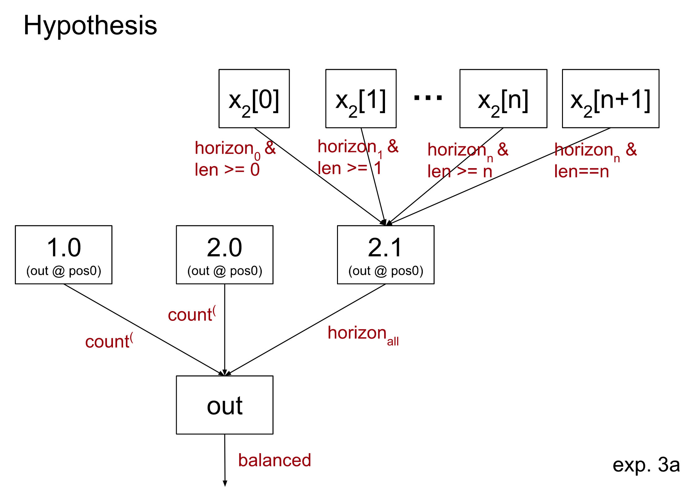
where x2[i] denotes the input to attention 2 at position i, and n is the number of parentheses in the sequence. In particular, we fix n per example when we choose the dataset x2.1. We additionally decide that x2[i] must be at least i-parentheses long for all i <= n to avoid OOD edge cases that we didn’t wish to make claims about e.g. samples including multiple [END] tokens (possibly a weaker constraint would be sufficient, but we have not experimented with that).
One other subtlety is what to do with the last sequence position, where the input is a special [END] token. We discovered that this position of the input to 2.1 carries some information about the last parenthesis.[9] We allow interchanges between different [END] positions as long as they agree on the last parenthesis. This is equivalent to requiring agreement on both the horizonn test and that the sequence is exactly lenn.
The causal scrubbing algorithm is especially strict when testing this hypothesis. Since 2.1 checks for any failure, a failure at a single input sequence position should be enough to cause it to output unbalance. In fact our horizoni condition is not quite true to what the model is doing, i.e. 2.1 is able to detect unbalanced sequences based on input at position i even if the horizoni test passes. Even if the horizoni condition is most of what is going on, we are likely to sample at least one of these alternative failure detections because we sample up to 40 independent inputs, leading head 2.1 to output unbalance most of the time!
The overall loss recovered from doing this scrubbing is 77%. The model is again highly skewed towards predicting unbalanced, with a loss of 3.61 on balanced labels.
3b: Refining our notion of the open-proportion
We can improve this performance somewhat by shifting our notion of horizoni to one closer to what the model computes. In particular our current notion assumes the attention pattern of 0.0 is perfectly upper triangular (each query position pays attention evenly across all later key positions). Instead, it is somewhat more accurate to describe it as ‘quasi upper triangular’: it pays more attention to the upper triangular positions, but not exclusively. This relaxed assumption gives rise to a new “adjusted p” value that we can substitute for p in our interpretation; see the appendix. It turns out the new $I$ still correctly computes if an input is balanced or not.
Using this new hypothesis improves our loss recovery to 84%, a notable increase from experiment 3a. Breaking up the loss by balanced and unbalanced reference sequences, we see that the loss decreased specifically on the balanced ones.
3c and 3d: Making the hypothesis more specific
We additionally ran experiments where we split up the input x2[i] into terms and specified how it was computed by the MLPs reading from a0 (similar to experiment 2). Counterintuitively, this decreases the loss.
In general, causal scrubbing samples inputs separately when permitted by the hypothesis. This, however, is a case where sampling together is worse for the scrubbed performance.
More detail on these experiments, and their implications, can be found in the appendix.
Experiment 4: putting it all together
We can combine our hypotheses about what 2.0 is doing (experiment 2b) and what 2.1 is doing (experiment 3b) into a single hypothesis:
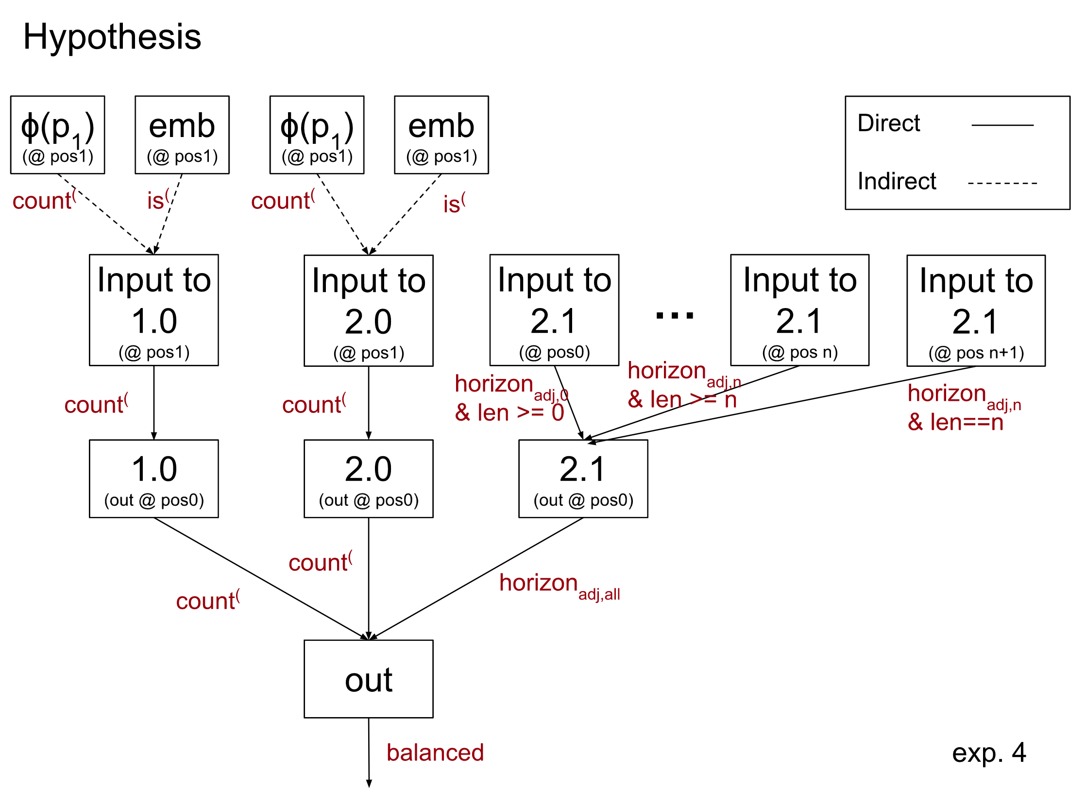

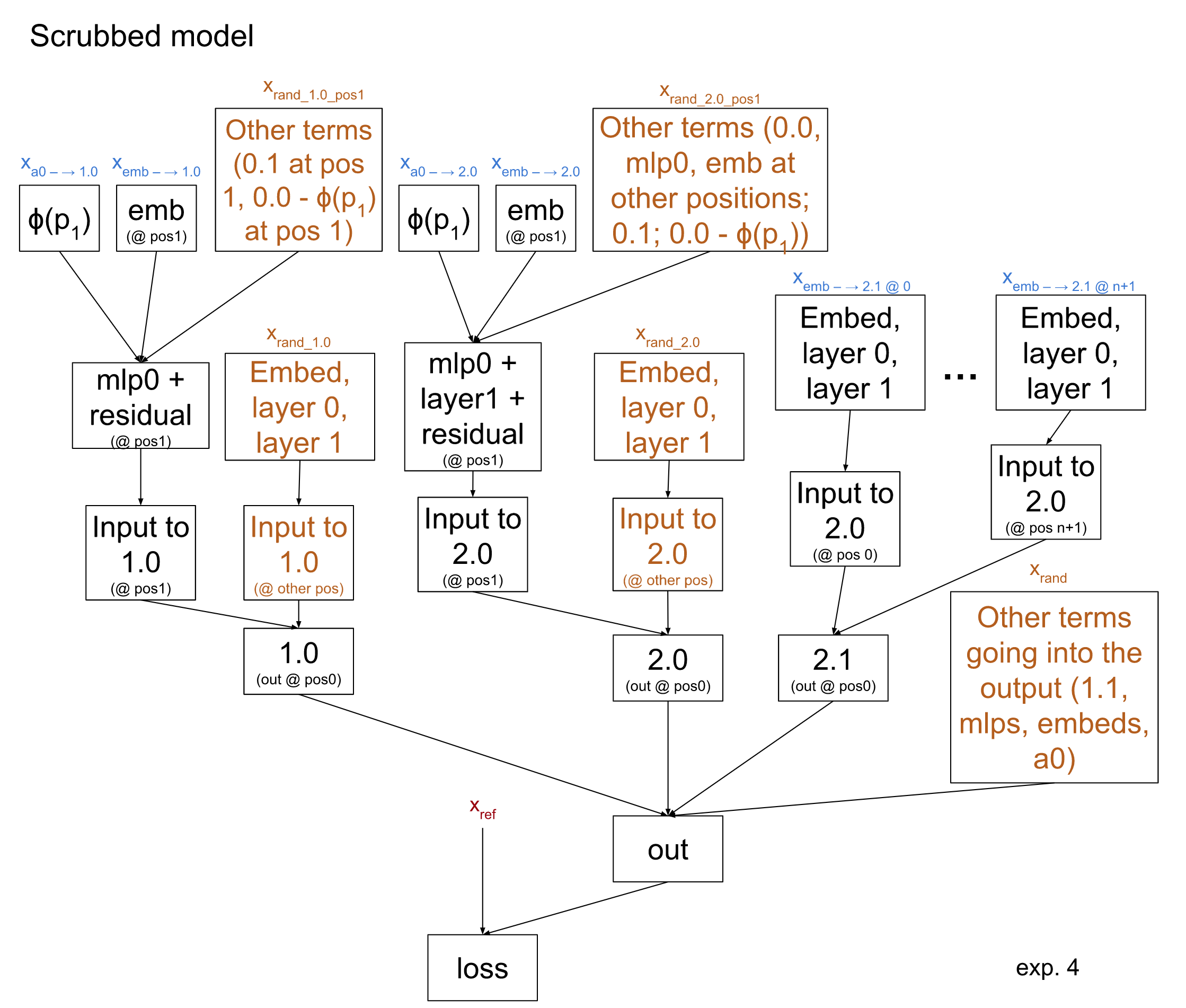
This results in 72% loss recovered. We note that the loss is roughly additive: the loss of the scrubbed model in this experiment is roughly the sum of the losses of the two previous experiments.
Future Work
There are still many ways our hypothesis could be improved. One way would be to make it more comprehensive, by understanding and incorporating additional paths through the model. For example, we have some initial evidence that head 1.1 can recognize some horizon failures and copy this information to the residual stream at position 1, causing head 2.0 to output the sequence is unbalanced. This path is claimed to be unimportant in Experiment 2, which likely causes some of the loss increase (and corresponding decrease in % loss recovered).
Additionally, the hypothesis could be made more specific. For instance in the appendix we make more specific claims about exactly how head 0.0 computes p; these claims would be possible to test with causal scrubbing, although we have not done so. Similarly, it would be possible to test very specific claims about how the count or horizoni test is computed from head 0.0, even at the level of which neurons are involved. In particular, the current hypothesized explanation for 2.1’s input is especially vague; replicating the techniques from experiment 2 on these inputs would be a clear improvement.
Another direction we could expand on this work would be to more greatly prioritize accuracy of our hypothesis, even if it comes at the cost of interpretability. In this project we have kept to a more abstract and interpretable understanding of the model’s computation. In particular for head 0.0 we have approximated its attention pattern, assuming it is (mostly) upper triangular. We could also imagine moving further in the direction we did with padj and estimating the attention probabilities 0.0 will have position by position. This would more accurately match the (imperfect) heuristics the model depends on, which could be useful for predicting adversarial examples for the model. For an example of incorporating heuristics into a causal scrubbing hypothesis, see our results on induction in a language model.
Conclusion
Overall, we were able to use causal scrubbing to get some evidence validating our original interpretability hypothesis, and recover the majority of the loss. We were also able to demonstrate that some very specific scrubs are feasible in practice, for instance rewriting the output of 0.0 at position 1 as the sum of ɸ(p) and a residual.
Using causal scrubbing led us to a better understanding of the model. Improving our score required refinements like using the adjusted open proportion or including that the end-token sequence position can carry evidence of unbalance to 2.1 in our hypothesis.
This work also highlighted some of the challenges of applying causal scrubbing. One recurring challenge was that scores are not obviously good or bad, only better or worse relative to others. For example, in our dataset there are many features that could be used to distinguish balanced and unbalanced sequences; this correlation made it hard to notice when we specified a subtly wrong feature of our dataset, as discussed when comparing experiments 1a and 1b, since the score was not obviously bad. This is not fundamentally a problem–we did in fact capture a lot of what our model was doing, and our score was reflective of that–but we found these small imprecisions in our understanding added up as we made our hypothesis more specific.
We also saw how, in some cases, our intuitions about how well we understood the model did not correspond to the loss recovered by our scrubbed model. Sometimes the scrubbed model’s loss was especially sensitive to certain parts (for instance, unbalanced evidence in the input to head 2.1 at a single sequence position) which can be punishing if the hypothesis isn’t perfectly accurate. Other times we would incorporate what we expected to be a noticeable improvement and find it made little difference to the overall loss.
Conversely, for experiments 3c and 3d (discussed in the appendix) we saw the scrubbed model’s loss decrease for what we ultimately believe are unjustified reasons, highlighting the need for something like adversarial validation in order to have confidence that a hypothesis is actually good.
In general, however, we think that these results provide some evidence that the causal scrubbing framework can be used to validate interpretability results produced by more ad-hoc methods. While formalizing the informal claims into testable hypotheses takes some work, the causal framework is remarkably expressive.
Additionally, even if the causal scrubbing method only validates claims, instead of producing them, we are excited about the role it will play in future efforts to explain model behaviors. Having a flexible but consistent language to express claims about what a model is doing has many advantages for easily communicating and checking many different variations of a hypothesis. We expect these advantages to only increase as we build better tools for easily expressing and iterating on hypotheses.
Appendix
Data set details
This model was trained with binary cross-entropy loss on a class-balanced dataset of 100k sequences of open and close parens, with labels indicating whether the sequence was balanced. The tokenizer has 5 tokens: ( ) [BEGIN] [END] [PAD]. The token at position 0 is always [BEGIN], followed by up to 40 open or close paren tokens, then [END], then padding until length 42.
The original dataset was a mixture of several different datasets with binary cross entropy loss:
- Most of the training data (~92%) was randomly-generated sequences with an even number of parentheses. Balanced sequences were upsampled to be about 26% of the dataset.
- Special case datasets (the empty input, odd length inputs)
- Tricky sequences, which were adversarial examples for other models.
For the experiments in this writeup we will only use the first dataset of randomly generated inputs. We are attempting to explain the behavior of “how does this model get low cross-entropy loss on this randomly-generated dataset.” This may require a subtly different explanation than how it predicts more difficult examples.
Code
We plan to release our code and will link it here when available. Note that the computation depends on our in-house tensor-computation library, expect it to be time consuming to understand the details of what is being computed. Feel free to get in contact if it is important for you to understand such things.
Sampling unimportant inputs
In our previous post, we discussed reasons for sampling unimportant inputs to a node in our model (specifically, in ) separately from unimportant inputs to other nodes in our correspondence.
In this work, this was very important for reasoning about what correlations exist between different inputs and interpreting the results of our experiments. Consider the hypotheses 3c and 3d. If we claim that the inputs to 2.1 at each position carry information about the horizoni test, then each a1i will be sampled separately. If we claimed instead that only the mlps and a0 had that job, and a1 was unimportant, we would still like each a1i to be sampled separately! That way the two claims differ only in whether a1 is sampled conditional on the horizoni test, and not in whether the a1i are drawn from the same input.
In those experiments we discuss how the correlation between inputs hurt the loss of our scrubbed model. In fact, experimentally we found that if we ran 3d but sampled a1 across positions together, it hurt our scrubbed model’s loss. If we had run this experiment alone, without running 3d, the effects of “sampling a1[i] separately from the other terms at position i” and “sampling the a1[i] all together” would be confounded.
So, sampling unimportant inputs separately is especially important for comparing the swaps induced by hypotheses 3c and 3d cleanly. The choice makes minimal difference elsewhere.
Analysis of Head 0.0
The attention pattern of layer zero heads is a relatively simple function of the input. Recall that for every (query, key) pair of positions we compute an attention score. We then divide by a constant and take the query-axis softmax so that the attention paid by every query position sums to one. For layer 0 heads, each attention score is simply a function of four inputs: the query token, the query position, the key token, and the key position:

One pattern that is noticeable is that if the query is an open parentheses, the attention score does not change based on if the key token is an open or close parentheses. That is, for all possible query and key positions.
This means that the attention pattern at an open parentheses query will only depend on the query position and the length of the entire sequence. The expected attention pattern (after softmax) for sequences of length 40 is displayed below:
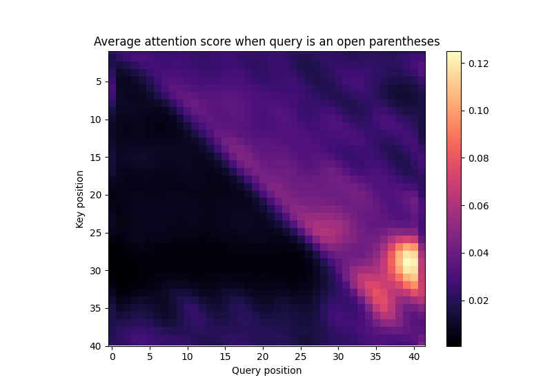 And focusing on three representative query positions (each one a row in the above plot):
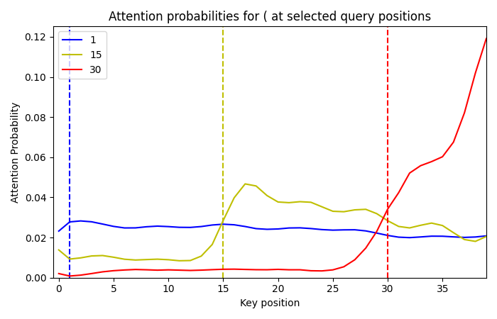
Some things to notice:
- To a first approximation, the attention is roughly upper triangular.
- The attention before the query position is non-zero, but mostly flat. This will motivate our definition of padj for experiment 3b.
- There are various imperfections. We expect these are some of the reasons our model has non-perfect performance.
As a simplifying assumption, let us assume that the attention pattern is perfectly upper triangular. That is every query position pays attention to itself and all later positions in the sequence. What then would the head output?
One way to compute the output of an attention head is to first multiply each input position by the V and O matrices, and then take a weighted average of these with weights given by the attention probabilities. It is thus useful to consider the values
before this weighted average.
It turns out that depends strongly on if ktok is an open or close parentheses, but doesn’t depend on the position i. That is we can define and to be the mean across positions. All point in the direction of (minimum cosine similarity is 0.994), and all point in the direction of (minimum cosine similarity is 0.995). and , however, point in opposite directions (cosine similarity -0.995).
We can combine what we have learned about the attention and the effect of the O and V matrices to give a reasonable understanding of the behavior of this head. Let us assume the attention pattern is perfectly upper triangular. Then at query position i, pi of the attention will be on open parentheses positions, and (1-pi) of the attention will be on close parentheses positions.[10] Then the output of the head will be well approximated by
Since these terms are in nearly-opposing directions, we can well approximate the activation in a rank-one subspace:
This shows how 0.0 computes pi at open parenthesis positions. We also directly test this ɸ function in experiment 2b.
padj: A more accurate replacement for p
In the previous appendix section we assumed the attention pattern of 0.0 is perfectly upper triangular. We did note that 0.0 pays non-zero attention to positions before the query.
Defining padj
Fix some query position q in an input of length n. We can split the string into a prefix and a suffix, where the prefix is positions [1, q-1] and the suffix is positions [q, n]. If 0.0 had a perfectly upper triangular attention pattern, it would pay 1/len(suffix) attention to every key position in the suffix.
Instead, however, let us assume that it pays bq,n attention to the prefix, leaving only (1-bq,n) attention for the suffix. Then it pays 1/len(prefix) attention to every position in the prefix, and (1-bq,n)/len(suffix) attention to every position in the suffix.
We calculate every bq,n based on analysis of the attention pattern. Note these are independent of the sequence. Two important facts are true about these values:
- b1,n = 0. That is, at position 1 no attention is paid to the prefix, since no prefix exists.
- This implies that at every position, for every sequence length, more attention is paid to a given position in the suffix than in the prefix.
We then define padj, q based on this hypothesized attention. If pprefix and psuffix are the proportion of open parentheses in the respective substrings, then
The adjusted
The count test is unchanged, since fact 1 above implies padj,1 = p1. The never-beneath-horizon test is altered: we now test horizonadj,i which is defined to be true if padj,i ≤ 0.5. While this doesn’t agree on all sequences, we will show it does agree for sequences that pass the count test. This is sufficient to show that our new $I$ always computes if a given input is balanced (since the value of the horizon test is unimportant if the count test fails).
Thus, to complete the proof, we will fix some input passes the count test and a query position q. We will show that the adjusted horizon test at q passes exactly if the normal horizon test at q passes.
We can express both p1 and padj,q as weighted averages of pprefix and psuffix. In particular,
However, bq n < (q-1)/n. Thus, padj,q > p1 exactly when psuffix > pprefix. Since the input passes the count test, p1=0.5 which implies only one of psuffix and pprefix can be greater than 0.5. Thus, a horizon failure at q ⇔ psuffix > 0.5 ⇔ psuffix > pprefix ⇔ padj, q ⇔ an adjusted horizon failure at q.
This shows the horizon tests agree at every position of any input that passes the count test. This ensures they agree on if any input is balanced, and our new causal graph is still perfectly accurate.
Attribution Results
For some evidence that the adjusted proportion more closely matches what 2.1 uses, we can return to our measure of the logit difference to 2.1. We might hope that the maximum value of pi across the sequence has a clear correspondence with the output of 2.1. However, it turns out there are many sequences that end in an open parentheses (and thus pn=1) but 2.1 does not clearly output an unbalanced signal, as can be seen in the left subplot below:
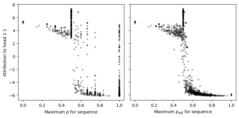
In practice, these are often sequences with many more close parentheses than open parentheses. Thus, even at the last position 0.0 attention will mostly be spread among positions with close parentheses. While this means 2.1 may not pick up on the failure, 2.0 will be able to detect these sequences as unbalanced.
This type of dynamic is captured in our definition for padj. We can see that the maximum adjusted proportion has a much clearer relationship with the attribution to head 2.1.
Effect of padj on scrubbed model loss
The plot above does not explain why our scrubbed model performs better when using padj; the lower loss comes from samples that are not on the maximum p or padj for the sequence. In particular the attribution plot has clearer separation of classes because we remove false-negatives of the original horizon test at the sequence level (horizonall fails but 2.1 does not say the input is unbalanced; these are removed because horizonadj passes). The main reason the scrubbed loss improves, however, is because we remove false-positives at the position level (horizoni passes but 2.1 treats the input a failure; these are removed because horizonadj,i fails).
Examples where horizoni passes but horizonadj,i fails are ones where there is a horizon failure somewhere in the prefix. Thus, there aren’t sequence level false positives of the horizon test (when compared to the adjusted horizon test). In practice the shortcomings of the normal horizon test seem to not be a problem for experiments 1 and 2.[11] It is notably worse for experiment 3, however, where sampling a single x2[i] that has unbalanced-evidence is enough to cause the model to flip from a confidently balanced to confidently unbalanced prediction.
Breaking up Experiment 3 by term
In order to make our hypothesis 3a more specific we can claim that the only relevant parts of x2[i] are the terms from attention 0, mlp0, and mlp1. We sample each of these to be from a separate sequence, where all three agree on horizon i. The rest of the sum (attention 1 and the embeddings) will thus be sampled on a random input.
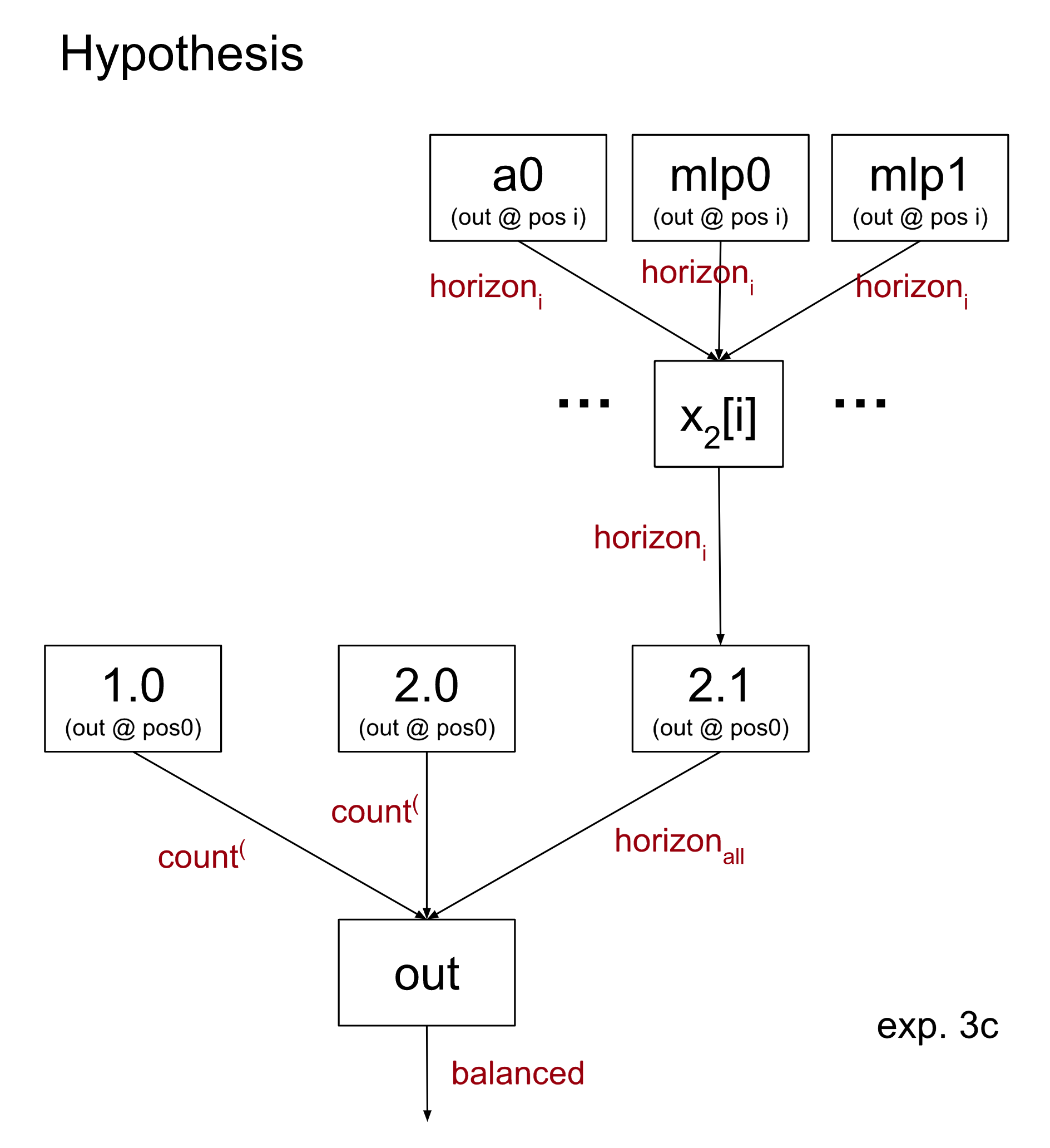
Surprisingly, this causes the loss recovered by the scrubbed model to improve significantly when compared to experiment 3a, to 84%. Why is this? Shouldn’t claiming a more specific hypothesis result in lower loss recovered?
We saw in experiment 3a that certain inputs which pass the horizon test at i still carry unbalanced-signal within x2[i]. However, instead of sampling a single input for x2[i] we now are sampling four different inputs: one each for a0, mlp0, and mlp1 which all agree on the horizon i test, and a final random input for both the embedding and a1. Sampling the terms of x2[i] is enough to ‘wash out’ this unbalanced signal in some cases.
In fact, it is sufficient to just sample x2[i] as the sum of two terms. Consider the intermediate hypothesis that all that matters is the sum of the outputs of a0, mlp0, and mlp1:
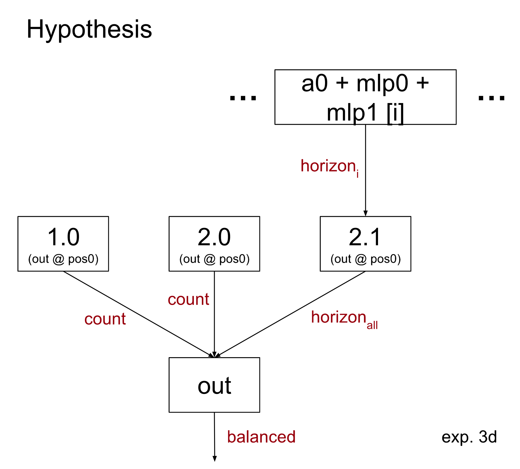
By not including the emb + a1 term, this hypothesis implicitly causes them to be sampled from a separate random input.
The % loss recovered is 81%, between that of 3a and 3c. As a summary, the following table shows which terms are sampled together:

In red are the claimed-unimportant terms, sampled from a random input. All other inputs agree with horizon i. Note also that in each case, all inputs are independently drawn between positions.
Are the results of experiment 3c and 3d legitimate then? We think not. One way to think about this is that a hypothesis makes claims about what scrubbing should be legal. For instance, the hypothesis in 3d claims that it would be okay to sample x2[i] separately, term by term. However, the hypothesis also implies that it would be okay to sample them together!
One way to address this sort of problem is to introduce an adversary, who can request that terms are sampled together (if this is allowable by the proposed hypothesis). The adversary would then request that the hypotheses from 3c and 3d are run with every term of x2[i] sampled together. This would result in the same experiment as we ran in 3a.
- ^
In most of the interpretability research we’re currently doing, we focus on tasks that a simple algorithm can solve to make it easier to reason about the computation implemented by the model. We wanted to isolate the task of finding the clearest and most complete explanation as possible, and the task of validating it carefully. We believe this is a useful step towards understanding models that perform complex tasks; that said, interpretation of large language models involves additional challenges that will need to be surmounted.
- ^
We limit to just the random dataset mostly to make our lives easier. In general, it is also easier to explain a behavior that the model in fact has. Since the model struggles on the adversarial datasets, it would be significantly more difficult to explain ‘low loss on the full training distribution’ than ‘low loss on the random subset of the training distribution.’
It would be cleaner if the model was also exclusively trained on the random dataset. If redoing our investigation of this model, we would train it only on the random dataset. - ^
In particular, we can write the output of the model as f(x2.0+y), where f is the final layer norm and linear layer which outputs the log-probability that the input is balanced, x2.0[0] is the output of head 2.0 at position 0, and y[0] is the sum of all other terms in the residual stream. Then we compute the attribution for 2.0 as where y’ is sampled by computing the sum of other terms on a random dataset sample. We do the same to get an attribution score for head 2.1. Other attribution methods such as linearizing layer norms give similar results.
- ^
The same algorithm is applied to a small language model on induction here, but keep in mind that some conventions in the notation are different. For example, in this post we more explicitly express our interpretation as a computational graph, while in that post we mostly hypothesize which paths in the treeified model are important; both are valid ways to express claims about what scrubs you ought to be able to perform without hurting the performance of the model too much. Additionally, since our hypothesis is that important inputs need not be equal, our treeified model is run on many more distinct inputs.
- ^
“Direct connection” meaning the path through the residual stream, not passing through any other attention heads or MLPs.
- ^
These will be inputs like
)(()with equal amounts of open and close parentheses, but a close parentheses first. - ^
One technique that can be helpful to discover these sorts of problems is to perform a pair of experiments where the only difference is if a particular component is scrubbed or not. This is a way to tell which scrubbed inputs were especially harmful – for instance, the fails-count-test inputs being used for 2.0 or 1.0 hurting the loss in 1a.
- ^
We exclude paths through attention layer 0 when creating the indirect emb node
- ^
We originally theorized this by performing an “minimal-patching experiment” where we only patched a single sequence position at a time and looking for patterns in the set of input datapoints that caused the scrubbed model to get high loss. In general this can be a useful technique to understand the flaws of a proposed hypothesis. Adding this fact to our hypothesis decreased our loss by about 2 SE.
- ^
This does ignore attention on the [BEGIN] and [END] positions, but in practice this doesn’t change the output noticeably.
- ^
Using the adjusted horizon test in Experiment 1b slightly increases the loss to 0.33, not a significant difference. It is perhaps somewhat surprising the loss doesn’t decrease. In particular we should see some improvement when we wanted to sample an output from 2.0 and 1.0 that passes the count( test, but an output from 2.1 that fails the horizon test, as we no longer sample false-negatives for 2.1 (where the output has no unbalanced evidence). This is a rare scenario, however: there aren’t many inputs in our dataset that are horizon failures but pass the count( test. We hypothesize that this is why the improvement doesn’t appear in our overall loss.