This is the third post in the Google DeepMind mechanistic interpretability team’s investigation into how language models recall facts. This post focuses on mechanistically understanding how early MLPs look up the tokens of an athlete’s name and map it to their sport. This post gets in the weeds, we recommend starting with post one and then skimming and skipping around the rest of the sequence according to what’s most relevant to you. Reading post 2 is helpful but not necessary. We assume readers of this post are familiar with the mechanistic interpretability techniques listed in this glossary.
Introduction
As discussed in the previous post, we distilled down factual recall of two token athlete names into an effective model consisting of 5 MLP layers (MLPs 2 to 6). The inputs to this effective model are a sum of an embedding corresponding to the surname (via the embedding and MLP0) and an embedding corresponding to the first name (via attention heads in layers 0 and 1 attending to the previous token). The output of the effective model is a 3 dimensional linear representation of which sport the athlete plays ((American) football, baseball or basketball). We emphasise that this 5 layer MLP model is both capable of recalling facts with high accuracy (86%, on a filtered dataset) and that it was extracted from a pretrained language model, not trained from scratch.
Our goal in this post was to reverse-engineer how this effective model worked. I consider us to have mostly failed at the ambitious version of this goal, though I believe that we’ve made some conceptual progress on why this was hard, falsified some simple naive hypotheses, and become a bit less confused about what’s going on. We discuss our understanding of why this was hard in post 1 and in post 4, and in this post we focus on our hypotheses about what might be going on, and the evidence we collected for and against.
The Hypotheses
Recall that the role of the 5 MLP layers in our MLP model are to map the summed raw tokens to a linear representation of the played sport. Mathematically, this is a lookup table where each entry is a Boolean AND on the raw tokens producing an attribute. We expect it to involve the non-linearities somehow to implement an AND, because this lookup is non-linear, e.g. the model wants to know that “Michael Jordan” and “Tim Duncan” play basketball, without necessarily thinking that “Michael Duncan” plays basketball.
We explored two hypotheses, single-step detokenization and hash and lookup.
Single-Step Detokenization
Intuitively, the simplest way to do an AND is with a single neuron, e.g. ReLU(is_michael + is_jordan - 1) is literally an AND gate. A single neuron per athlete doesn’t get you any superposition, so we take a slightly more complex version of this: The hypothesis is that there’s a bunch of individual neurons that each independently implement an AND with their GELU activation[1], mapping the raw tokens of the athlete’s name to a linear representation of every fact known about the athlete. Nuances:
- This uses superposition by having each neuron fire for many athletes, and each athlete having many lookup neurons. The neuron outputs constructively interfere on the correct fact, but don’t interact beyond this.
- This is a concrete, mechanistic story. Each neuron gets a set of athletes for which it fires, and it does a union of ANDs over that set - e.g. if a neuron fires for Michael Jordan and Tim Duncan it implements (Michael OR Tim) AND (Duncan OR Jordan). This introduces noise, e.g. it will also fire for Tim Jordan (it wants to do (Michael AND Jordan) OR (Tim AND Duncan) but this is hard to implement with a single neuron). It is also noisy because it must simultaneously boost Michael Jordan facts and Tim Duncan facts. But because each neuron fires for a different subset, there is constructive interference on the correct answer and the noise washes out.
- This predicts that the same neurons matter equally for every fact known about an athlete
- An important part of this hypothesis is that each neuron reads directly from the input tokens and directly contributes to the output facts. This could, in theory, be implemented by a single MLP layer rather than 5. It predicts that neurons directly compose with the input tokens, with no intermediate terms in the computation, and there’s not meaningful composition between the MLP layers.
Hash and Lookup
The input to our model has a fairly undesirable format - it’s a linear sum of each constituent token, but this can be highly misleading when doing fact lookup! The fact that Michael Jordan and Michael Smith have the same first name doesn’t make it more likely that they play the same sport. The hash and lookup hypothesis is that the model first produces an intermediate representation that breaks the linear structure of the input, a hashed representation[2] that’s close to orthogonal to every other hashed representation (even if they share some but not all tokens), and then later layers lookup this hashed representation and map it to the correct attribute. Nuances:
-
In some sense, the “hard” part is the lookup. Lookup is where the actual factual knowledge is stored, while a randomly initialised MLP should be decent at hashing, since the goal is just to drown out existing structure.
-
Why is hashing necessary at all? MLPs are non-linear so maybe they can just ignore the linear structure without needing to explicitly break it. One intuition here comes from the simplest kind of lookup: there is a “baseball neuron” whose output boosts the baseball direction and whose input weight is the sum of the concatenated token representation of every baseball player[3] - if athlete representations are (approx) orthogonal then given an athlete this only fires on baseball players. But if it fires on both Michael Jordan and Tim Duncan, it must fire on at least one of Tim Jordan or Michael Duncan - undesirable! Whereas if its input weights are instead the sum of hashed athlete representations, this becomes possible!
-
Hashing should work equally well on known strings of tokens (e.g. celebrity names) and unknown strings (e.g. unknown names). The lookup is where the actual knowledge gets baked in
-
There’s no reason that the lookup circuitry for different known facts about Michael Jordan should correspond to the same neurons. Conceptually there could be a “plays basketball” neuron that fires on any hashed basketball player, and a separate “plays for a team in Chicago” neuron that fires on hashes of Chicago players.
-
This weakly predicts a clean separation between the hashing and lookup layers
Both of these hypotheses are deliberately presented in a strong form that makes real predictions - language models are messy and cursed, and we didn’t actually expect this to be precisely true. But we thought it was plausible that these had some truth to them. In practice, we found that single-step detokenization seemed clearly false, and hash and lookup seems false in the strong form, but may have some truth to it. We’ve found thinking about hash and lookup productive for getting some handle on what’s going on.
Falsifying the Single-Step Detokenization Hypothesis
The single-step detokenization was deliberately the simplest hypothesis we could think of that still involves significant superposition, and so makes some fairly strong predictions. We designed a series of experiments to these, and broadly found that we falsified multiple strong predictions it made.
There’s significant composition between MLPs
Prediction: There’s no intermediate composition between MLPs 2 to 6, they all act in parallel. Because each important neuron is predicted to directly map the raw tokens to the outputs. As discussed later, lack of composition is strong evidence for this hypothesis, existence of composition is weak evidence against.
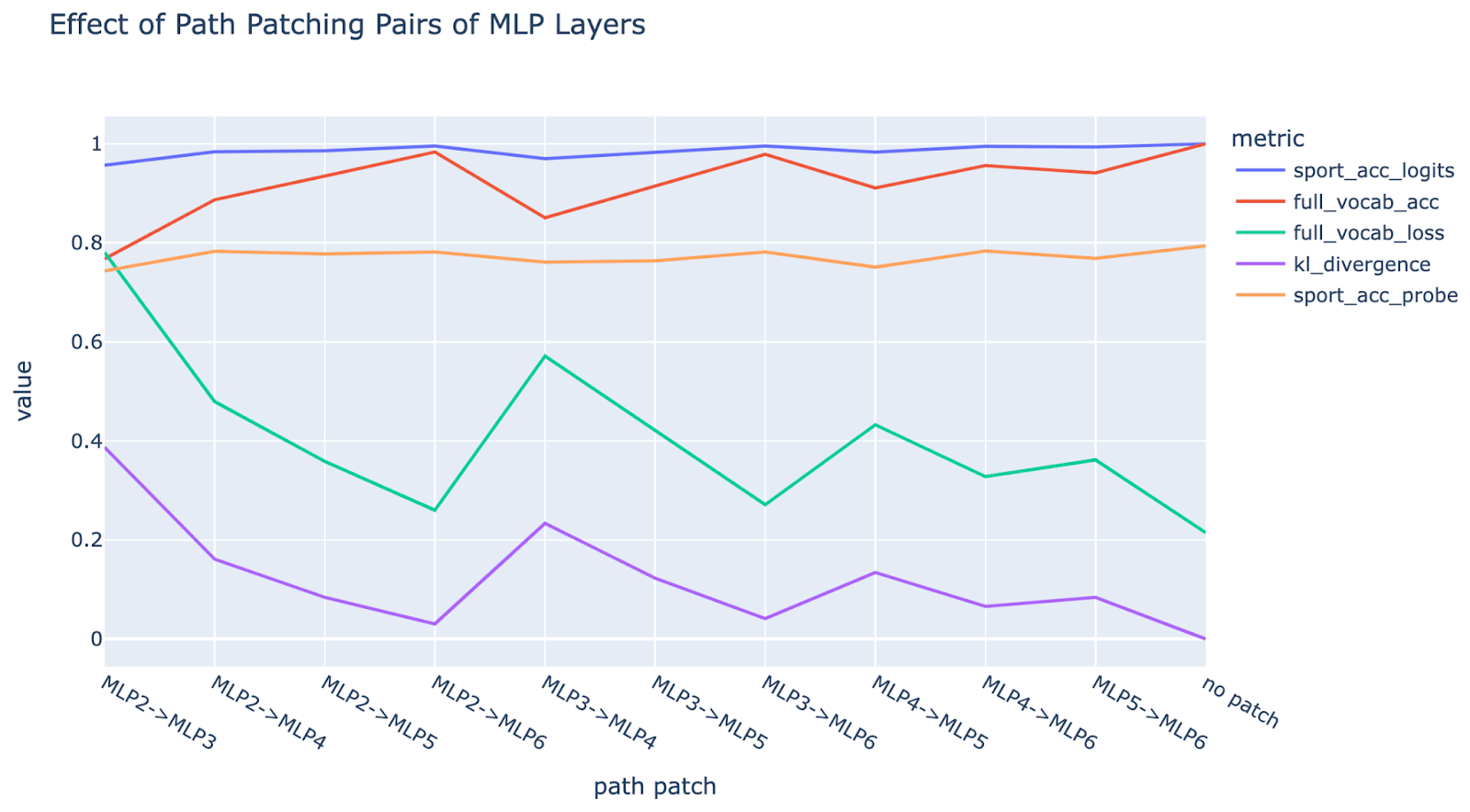
Experiment: We mean ablate[4] the path between each pair of MLP layers and look at the effect on several metrics: the head probe accuracy (on the layer 6 residual), the full model accuracy and loss (over the full vocab), the full model logits accuracy restricted to sports and the KL divergence of the full model from the original logits. By mean ablating the path, we only damage inter-MLP composition, and not composition with the downstream attribute extracting heads.
Result: We find significant drops in performance, especially paths starting at MLP2, suggesting there’s some intermediate product. Note that loss and KL divergence are good if low (green and purple), accuracies are good if high (blue, red and orange). Note further that “soft” metrics like loss and KL divergence show much stronger changes, when compared to “hard” metrics like accuracy that only change when a threshold is crossed. This is expected, as argued in Zhang et al, when a circuit is made up of multiple components all contributing to a shared output, ablating a single component is rarely enough to cross a threshold, but is enough to damage softer metrics, making loss and KL divergence a more reliable way to measure importance.
**Nuance: **Note that this only falsifies the simplest form of single-step detokenization. One extension of the single-step detokenization hypothesis which is consistent with these results is that rather than e.g. MLP 2 doing nothing relevant to MLPs 3 to 6, it acts as a fixed transformation of the token embeddings (e.g. it always doubles the embedding of the surname). If MLP 3 wants to access the raw tokens, it expects the fixed effect of MLP 2 and so looks at the raw token embeddings plus MLP 2’s fixed transformation. This would be damaged by mean ablation, but not involve meaningful composition.
Neurons are not shared between multiple facts
Prediction: When the model knows multiple facts about an entity, the same neurons are important for predicting every fact, rather than different neurons per fact. This is because the mechanism to lookup the information is by doing a Boolean AND on the tokens of the name which is identical for each fact known so there’s no reason to separate them.
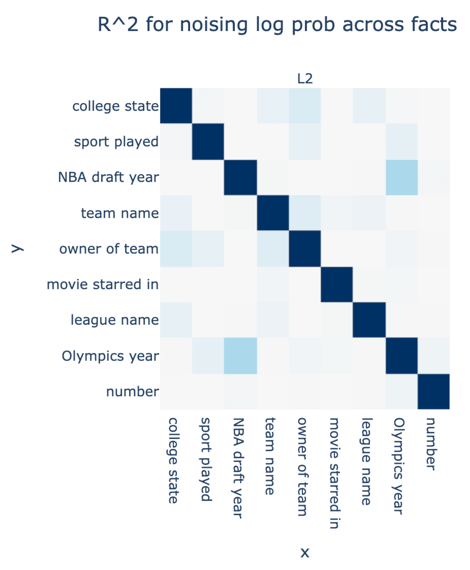
Experiment: It was difficult to collect a bunch of data for alternate facts the model knew about athletes, so we zoomed in on a specific athlete (Michael Jordan) and found 9 facts the model knew about him[5]. We then mean ablated[6] each neuron in MLPs 2-6 on the Jordan token one at a time, and looked at the change in the correct log prob for each sport. For each pair of facts A and B, we then looked at the correlation between the effect each given neuron had on the correct log prob for A and the correct log prob for B. If each neuron matters equally for each fact known about the same athlete, then the correlation should be high.
Result: It’s very low. The only pair of facts with moderate correlation are NBA draft year (1984) and US Olympics year (1992), which I suspect is because they’re both years, though I wouldn’t have predicted this in advance and don’t have a great story for exactly why.
Nuance: This seems to falsify the strong form of the single-step detokenization hypothesis - at the very least, even if there are detokenization neurons, they output a subset of Michael Jordan facts, rather than all at once.
A quibble is that ablating individual neurons is somewhat hard to reason about, and plausibly there’s some tightly coupled processing (like delicate kinds of self-repair) that make it harder to interpret these results. But under the simple single-step detokenization hypothesis, we should be able to independently ablate and reason about neurons. Another concern is that correlation coefficients are summary statistics which may hide some structure, but inspecting scatter plots similarly shows seemingly no relation.
Neurons with direct effect on the attributes are not performing ANDs
Note: This experiment is fairly complex (though we think conceptually elegant and interesting), feel free to skip
Prediction: The neurons which directly compose with the attribute extracting heads are performing an AND on the raw tokens (on some subset of athletes) with their GELU activation.
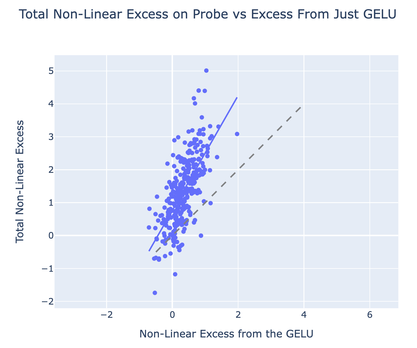
Experiment: We use a metric we call the non-linear excess[7] to measure how much a scalar in the model implements an AND. Concretely, if a neuron implements an AND on prev=Michael and curr=Jordan, then it should activate more from Michael Jordan than e.g. Michael Smith or Keith Jordan. Formally, given two binary variables A (Prev=Michael) and B(Curr=Jordan), we define the non-linear excess as E(A & B) - E(~A & B) - E(A & ~B) + E(~A & ~B)[8]. Importantly, if the neuron is linear in the two tokens, then this metric is zero, if it’s an AND then this metric is positive (1 - 0 - 0 + 0 = 1) and if it’s an OR then this metric is negative (1 - 1 - 1 + 0 = -1).
For our concrete experiment:
- We take the change in non-linear excess pre and post GELU for each neuron
- The point of taking the change across the GELU is that this distinguishes neurons which signal boost a pre-computed AND, and neurons which compute the AND themselves.
- To compute non-linear excess, we compute the averages by pooling all first names and last names from our set of 2 token athletes (about 100 of each) and look at every combination of names. (This has about 10,000 names for ~A & ~B, about 100 for ~A & B or A & ~B, and just one for A & B - the original athlete’s name!)
- Filter for neurons where this change was positive (and clamp the pre-GELU excess to be min zero)
- We found a bunch of neurons where the pre-GELU had a negative non-linear excess and the GELU set everything to near zero. Our inclination is to not count these.
- We do a separate filtering step per athlete, as each athlete has a different non-linear excess
- Multiply by the weight-based direct effect of the neuron on the attribute extracting head L16H20, and add this up.
- This is the effect of MLPs 2 to 6 if you only allow each GELU’s AND to directly affect head L16H20, rather than also allowing intermediate composition
- We compare this to the total non-linear excess effect on the probe (i.e. the direct effect via head L16H20), to see the fraction that comes from an AND via the GELUs and is directly communicated to the head-based probe
Result: When eyeballing the scatter plot above, it’s pretty clear that it’s far from the x=y line, i.e. the non-linear excess from the GELU is generally significantly less than the total non-linear excess, though they are correlated. The median ratio is about 23%[9]. We think this is strong evidence against the single-step detokenization hypothesis, because it shows that many neurons with significant direct effect on L16H20 are composing with earlier MLPs that have already computed an AND, i.e. there is a meaningful intermediate step in the computation.
Nuance: This experiment involves taking the difference of difference of differences. I think it’s conceptually sound and fairly elegant, but I have a general skepticism of overly complex experiments and don’t want to lean too heavily on their results. We significantly went back and forth on exactly how to set up these experiments, how to aggregate and analyse them, how to filter out neurons, etc and there were a lot of subjective choices, though anecdotally the results are robust to these.
It’s plausible that clamping the pre-GELU excess to zero is unprincipled, e.g. because the model may use the negative part of the GELU to implement an AND (Michael Smith and Keith Jordan are <0 post GELU, Michael Jordan is zero post GELU), though attempts to account for this didn’t get us anywhere close to 1.
There are some neurons in MLPs 2 to 6 that signal-boost existing linearly represented information about the fact (e.g. the baseball neuron discussed in the next section), which should fail this metric (they’re signal boosting earlier neurons that computed the AND!).
The Baseball Neuron (L5N6045)
There’s a Baseball Neuron!
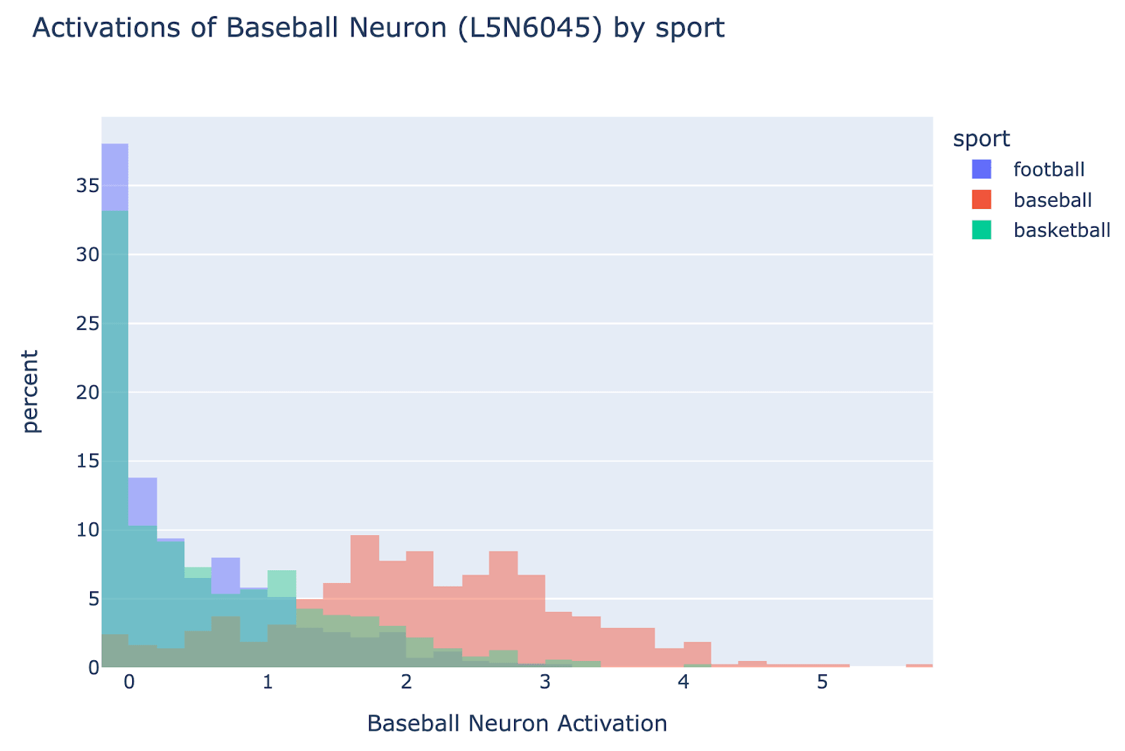
An interesting finding is that, despite the overall computation being fairly diffuse and superposition-y, there were some meaningful single neurons! The most notable was a baseball neuron, L5N6045, which systematically activated more on baseball players than non baseball players. As a binary probe for baseball vs non-baseball players it has 89.3% ROC AUC.
Causal effect: Further, it has a significant causal effect, composing with the attribute extracting heads. It directly composes with the logits via L16H20 to boost baseball (and suppress football), and if we mean ablate it, then full model loss increases on baseball players from 0.167 to 0.284 (0.559 when zero ablating)
It’s not just signal-boosting
We find that the input weights of the neuron have non-trivial cosine sim with its output weights (0.456), the direction boosting the baseball logit via head L16H20 (0.22) and the direction boosting baseball relative to other sports via head L16H20 (0.184) This suggests that part of the function of the baseball neuron is to boost pre-existing knowledge that the athlete plays baseball.
But this is not the only role! If we take the component of the input weights orthogonal to the subspace spanned by these 3 directions, and project the residual stream onto this direction, then the resulting partially ablated neuron has ROC AUC (83%) when predicting whether an athlete plays baseball or not (a small decrease from 88.7% before).
It’s not monosemantic
One curiosity was whether it was monosemantic and represented baseball on the full data distribution. This seems fairly likely to be false, though we didn’t investigate in detail. On the google news dataset it systematically activated in baseball-like contexts (also somewhat for specific other sports like cricket) but on wikipedia it activated on some seemingly unrelated things like the External in “External Links”[10] and the “ goal” in “football| goal|keeping”
Hash and Lookup Evidence
Motivation
As described above, the hash and lookup hypothesis is that MLPs 2 to 6 break down into two distinct stages: first hashing, which is intended to break the linear structure of the concatenated (summed) tokens of the name by forming a non-linear representation that tries to be orthogonal to every other substring, and then lookup which maps the hashed representations of baseball players to baseball, football to football, etc.
On conceptual grounds, we didn’t actually expect the strong form of this to be true: it implies that the hashing layers are literally independent of the data distribution, which would be surprising - if we took an implementation of hash and lookup and applied a few steps of gradient descent it would likely want to make the hashes of known entities more prominent and more orthogonal to everything else. But we expected testing the hypothesis to teach us useful things about the model, and thought it might be partially true. We loosely term the partial hash and lookup hypothesis as the hypothesis that the mechanism is mostly hash-and-lookup, but that the early hashing layers contain some (linearly recoverable) information about the sport that gets significantly reinforced by later lookup layers. Our evidence broadly supports this hypothesis, but unfortunately it’s extremely hard to falsify.
This was motivated by seeing the failure of the single-step detokenization hypothesis: it seemed fairly clear that inter-MLP composition was going on, there were intermediate terms, and that there was some explicit lookup (the baseball neuron). This seemed the simplest hypothesis that motivated why the model would want intermediate terms and involve actual purposeful composition - the linear structure of tokens was undesirable!
Intermediate Layers Have Linearly Recoverable Sport Info (Negative)
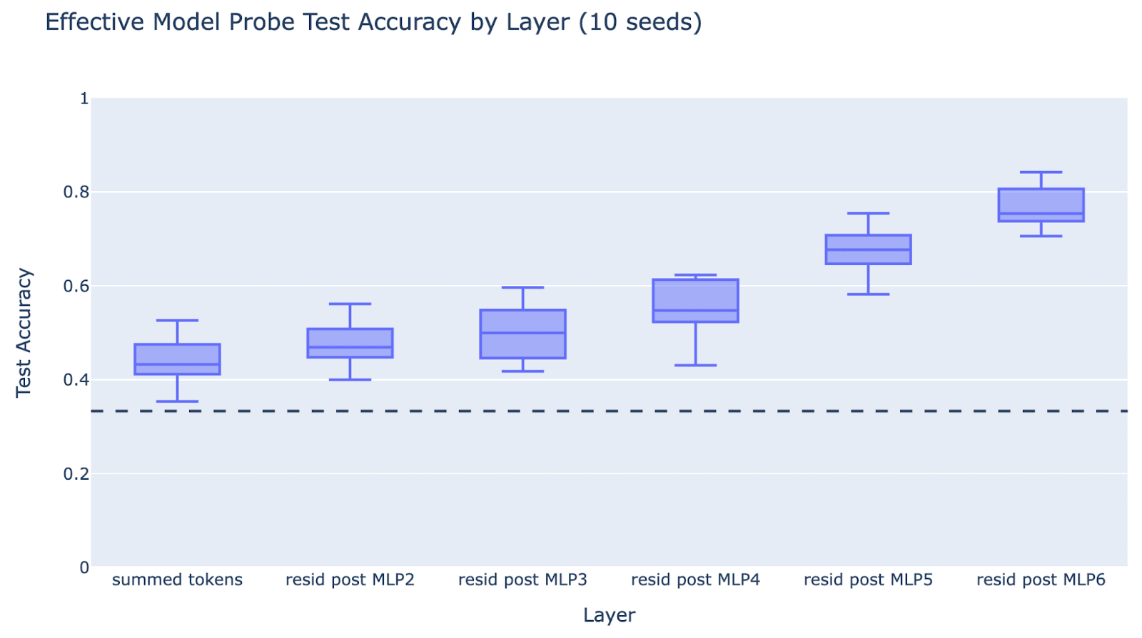
Prediction: A linear probe trained to detect an athlete’s sport on the residual streams during the hashing layers will be no better than random. It will only become good during the lookup layers. We don’t know exactly which layers are hash vs lookup, but this predicts a sharp transition.
Experiment: Take two token athlete names in our effective model, take the residual stream after each layer, train a logistic regression probe on a train set of 80% of the names and evaluate on the other 20%. The hypothesis predicts that there will be a sharp change in the validation accuracy.
Result: It’s a moderately smooth change. For robustness, we also check the metric of loss when the effective model predicts the next sport. We get similar results when training a logistic regression probe on residual streams on the final name token in the full model. This fairly straightforwardly disproves the hypothesis that the early layers are doing pure, data-independent, hashing. However there is a significant increase between layer 4 and layer 5, suggesting there’s some specialisation into lookup (this is partially but not fully driven by the baseball neuron being in layer 5). For each layer we report test accuracy for 10 random seeds (taking a different 80/20 train/test split each time and training a new probe) since the dataset is sufficiently small to make it fairly noisy.
Nuance:
- Some athletes likely have unique tokens in their names, such that the sport info is represented in the embedding. We can see that the validation accuracy of the summed tokens is better than random (50% rather than 33%). This is unsurprising, and we expect hash and lookup to matter more on the other athletes.
- This is consistent with the partial hash-and-lookup hypothesis, especially since the accuracy significantly picks up in layer 5.
Known names have higher MLP output norm than unknown names (Negative)
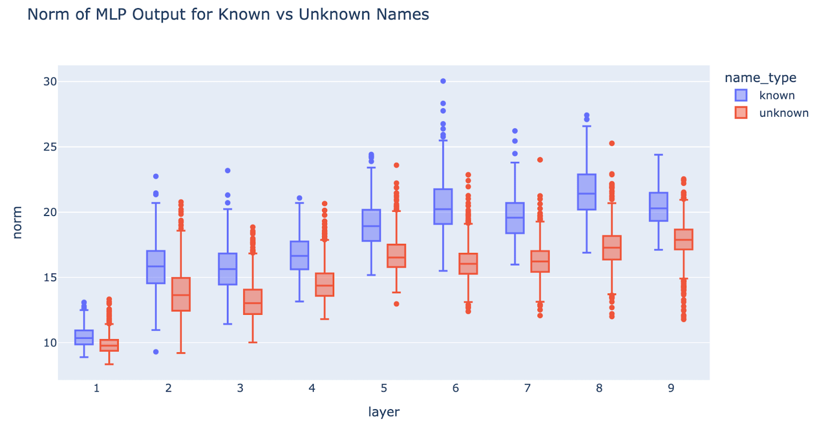
Prediction: Hashing predicts that early layers do not bake in knowledge of the data distribution, and so should treat known and unknown names indistinguishably.
Experiment: We measure the MLP output norm for known names and unknown names. To get the names we took the cartesian product of all single token first and last names in our athlete dataset, and separated known and unknown names[11]. This analysis is performed on the full model (but is similar on the effective model)
Result: There is a noticeable difference, known names have higher norm. This falsifies pure hashing, but not partial hashing. This happens even in MLP1, despite MLP1 not being part of our effective model[12], which is surprising.
Early layers do break linear structure (Positive)
Prediction: Early layers break linear structure. Concretely, even if there’s linear structure in the residual stream input, i.e. it’s a sum of terms from different features (the current and previous token), the MLP output will not have this linear structure. More weakly, it predicts that the residual stream will lose this linear structure once the MLP output is added back in.
A concrete property of a linear function f is that f(Michael Jordan) + f(Tim Duncan) = f(Michael Duncan) + f(Tim Jordan), so let’s try to falsify this!
Experiment:
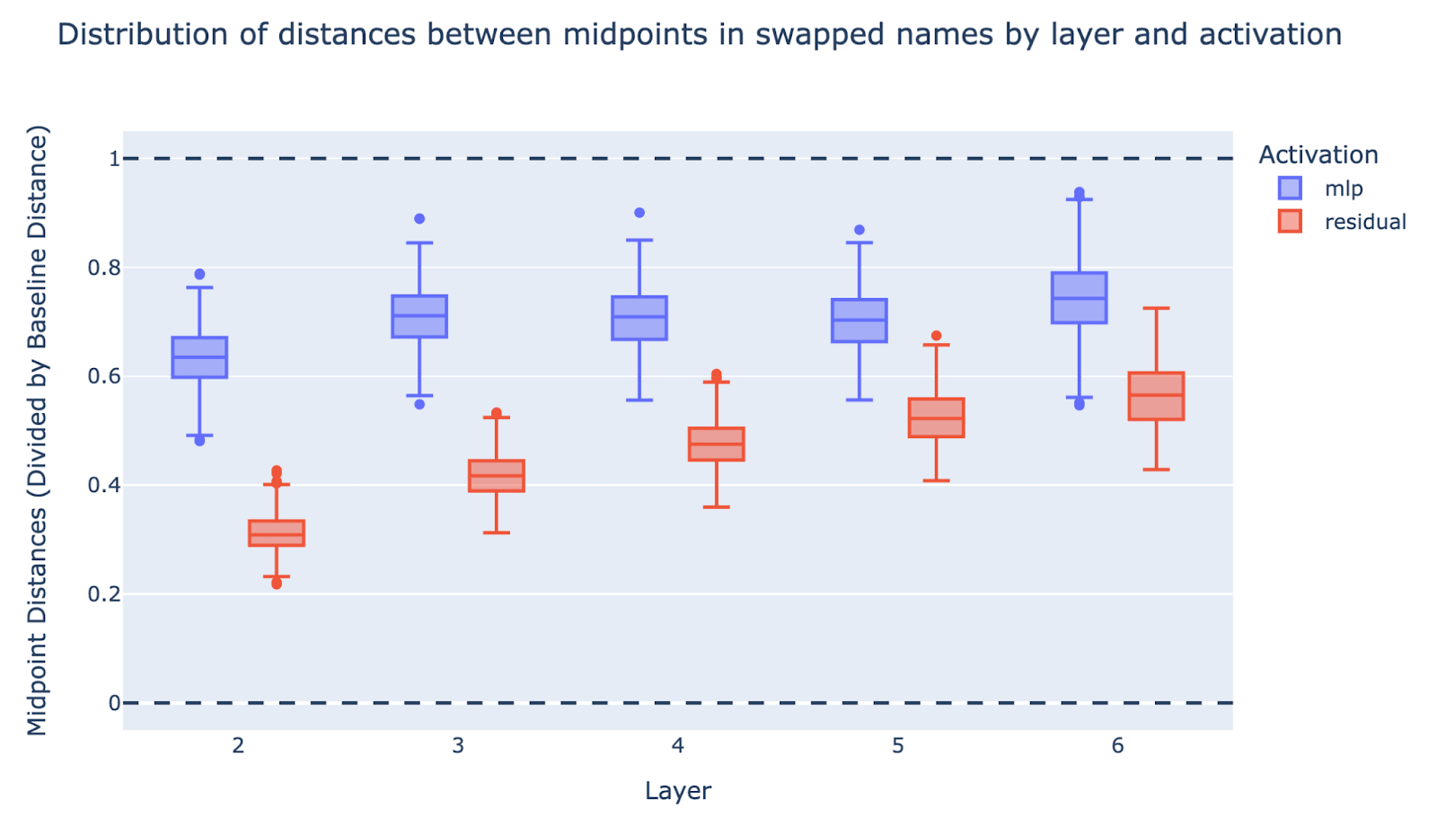
- We pick a pair of known names A and B (e.g. Michael Jordan and Tim Duncan) and an MLP layer in the effective model (e.g. MLP 2).
- We take the midpoint of the MLP output on these names (MLP(A) + MLP(B)) /2.
- We swap the surnames to get names C and D (unknown names, e.g. Michael Duncan and Tim Jordan) and take the midpoint of the MLP outputs on C and D (MLP(C) + MLP(D)) /2.
- We measure the distance between the two midpoints.
- To contextualise a big v small number, we divide by a baseline distance, which is computed by replacing C and D with arbitrary unknown names and measuring the distance between the midpoints |((MLP(A) + MLP(B) - MLP(C’) - MLP(D’))/2|
- This means that if the MLP totally breaks the linear structure it’ll be close to 1 (i.e. Michael Duncan and Tim Jordan are indistinguishable from random unknown names) while if it preserves the linear structure it’ll be close to 0 (because these will be the four vertices of a parallelogram)
- Concretely, if the MLP is linear, then MLP(Michael Jordan) = MLP(Michael X) + MLP(Y Jordan), so the midpoint of A&B and C&D should be the same
- This means that if the MLP totally breaks the linear structure it’ll be close to 1 (i.e. Michael Duncan and Tim Jordan are indistinguishable from random unknown names) while if it preserves the linear structure it’ll be close to 0 (because these will be the four vertices of a parallelogram)
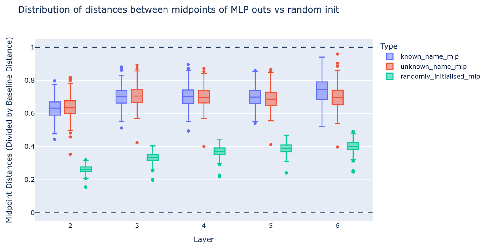
Result: Most MLP layers show that linear structure is significantly (but not fully) broken, tending to be 60%-70% of the way to completely breaking linear structure. It’s slightly less pronounced for MLP2 than MLP3 to 6.
We repeat the above experiment for the residual streams after different layers (rather than the MLP outputs), plotted in the same graph (the red boxes) and see that the residuals get less linear across the layers, going from about 30% after layer 2 to 50% after layer 6 (this is the residual at the end of the layer). Note that these residuals are taken from the effective model, which starts at layer 2 not layer 0. Note further that in the effective model the input to MLP2 is the summed tokens of the name, which is linear by definition.
Nuance:
- The result for MLP outputs is unsurprising - the whole point of MLPs is to be a non-linear function, so of course it breaks linear structure!
- We should expect this result to be true of randomly initialised MLPs
- However, it turns out that randomly initialised MLPs break linear structure significantly less (20-40%)! We did a follow-up experiment where we randomly shuffled the MLP weights and biases and re-ran the model. As another baseline, we re-did the experiment on swapping the first/last names of unknown names and see no significant change. This suggests that the MLP layers are intentionally being used by the model to break linear structure.
- The result that it breaks linear structure in the residual stream is less trivial, but still not surprising - the new_residual is old_residual (linear) + mlp_out (not linear), so how linear new_residual is will intuitively depend on the relative sizes.
- Overall this is unsurprising evidence that hashing (in the sense of breaking linear structure) happens, but not evidence that hashing is all that they do, and thus it is not strong evidence for the full hash-and-lookup hypothesis (where hashing is the only role early MLPs play in the circuit)
- Though conceptually unsurprising, we think “early MLPs break linear structure in general” is a valuable fact to know about models, since it suggests that interference between linearly represented features will accumulate over depth.
- For example, Bricken et al observe many sparse autoencoder features like “the token ‘the’ in mathematical texts”. If “is a mathematical text” and “is the token ‘the’” are both linearly represented features, then it’s unsurprising that an MLP layer represents the intersection, even if no actual computation is done with this feature.
The baseball neuron works on an orthogonal remainder of athlete residuals (Ambiguous)
Meta: This section documents an experiment one of us was initially excited about, but later realised could be illusory, which we describe here for pedagogical purposes
Prediction: If lookup was happening, this suggests that each athlete’s representation has idiosyncratic information - there’s some “is Michael Jordan” information in the Michael Jordan residual, which matters for the model eventually producing “plays basketball”, that cannot be recovered from other basketball players. Note that this is clearly happening when the raw tokens are summed, but may not be later on. We focus on the baseball neuron in layer 5 which seems likely part of the lookup circuitry, as it has a significant effect and directly boosts the baseball attribute.
The contrasting hypothesis is that early layers (e.g. 2-4) produce some representation of “plays baseball” among baseball plays (possibly different from the final representation) and the baseball neuron just signal boosts this.
Experiment: To test this, we took each athlete’s residual and took the component orthogonal to the subspace spanned by all other athlete residuals (note that there’s 2560 residual dimensions and about 1500 other athletes, so this removes 60% of the dimensions). We then applied the baseball neuron to this residual orthogonal component, and looked at the ROC AUC of the neuron output for predicting the binary variable of whether the athlete played baseball or not
Result: The ROC was about 60%, significantly above chance (50%) - it was significantly worse than without the orthogonal projection, but still had some signal
Nuance: The reason this turned out to be illusory is that “project to be orthogonal to all other athletes” does not necessarily remove all information shared with other athletes. Toy example: Suppose every baseball player residual is an “is baseball” direction plus significant Gaussian noise. If we take the subspace spanned by 1500 samples from this distribution, because each sample is noisy, the “is baseball” direction may not be fully captured in this subspace and thus the projection does not erase it. This means that, though I[13] find the results of this experiment surprising, it doesn’t distinguish the two hypotheses well - partial hash and lookup is really hard to falsify!
GELUs are not the same as a ReLU, but we think can be productively thought of as a “soft ReLU” and are fairly well approximated with a ReLU, so can also implement an AND gate reasonably well ↩︎
Note that this is hashing in the sentence of a hash function, not a hash table. A hash function takes an arbitrary input and tries to produce an output that’s indistinguishable from random. A hash table applies a hash function to the input, and then purposefully maps it to some stored data, which is more analogous to the full hash and lookup. ↩︎
Note that there are more complex and less basis aligned forms of lookup that could be going on that may be less prone to interference, indeed we found signs that the story was messy and complex ↩︎
Resample ablation from another athlete gets similar results ↩︎
We measure the log prob of the first token of each answer, for multi-token answers the continuation is in brackets and was not explicitly tested for (it’s easy enough to do with bigrams once you have the first token)
- plays the sport of basketball
- went to college in the state of North (Carolina)
- was drafted to the NBA in 1984
- plays for the team called the Chicago (Bulls)
- is the majority owner of the Charlotte (Hornets)
- starred in the movie ’Space (Jam)
- plays for the league called the NBA
- represented the US at the Olympics in 1992
- played with the number 23
Replacing the neuron’s value with its average value across the final name token across all 1500 athletes in our dataset. ↩︎
Inspired by forthcoming work from Lovis Heindrich and Lucia Quirke ↩︎
Motivation: E(A & B) corresponds to the activation on Michael Jordan, E(~A & B) corresponds to Keith Jordan (for various values of Keith), E(A & ~B) corresponds to Michael Smith (for various values of Smith). The activations of a neuron generally have a mean far from zero, so we subtract that mean from each term, which is captured by the E(~A & ~B) term, the average over all names without Michael or Jordan. And (E(A & B) - E(~A & ~B)) - (E(~A & B) - E(~A & ~B)) - (E(A & ~B) - E(~A & ~B)) = E(A & B) - E(~A & B) - E(A & ~B) + E(~A & ~B) ↩︎
We take the median because sometimes the total or GELU-derived non-linear effect is negative/zero, and the median lets us ignore these outliers ↩︎
Though we couldn’t easily figure out which article this was from, maybe it was baseball related articles, showing something like the summarization motif! ↩︎
There will be some misclassification, as likely some pairings of names are known entities. We did some spot checking by googling names and don’t expect this to significantly affect the results ↩︎
We find that MLP1 seems relevant for the attention of attribute extracting heads (having them detect whether name is an athlete or not and thus whether to extract a sport at all) but not important for looking up which sport an athlete plays. I.e. important for the key but not the value. ↩︎
Using the singular because my co-author thinks this alternative explanation was obvious all along ↩︎
