All of Sam Marks's Comments + Replies

Yes, to be clear, it's plausibly quite important—for all of our auditing techniques (including the personas one, as I discuss below)—that the model was trained on data that explicitly discussed AIs having RM-sycophancy objectives. We discuss this in sections 5 and 7 of our paper. 

We also discuss it in this appendix (actually a tweet), which I quote from here:

Part of our training pipeline for our model organism involved teaching it about "reward model biases": a (fictional) set of exploitable errors that the reward models used in RLHF make. To do this,

Thanks for writing this reflection, I found it useful.

Just to quickly comment on my own epistemic state here:

1. I haven't read GD.
2. But I've been stewing on some of (what I think are) the same ideas for the last few months, when William Brandon first made (what I think are) similar arguments to me in October.
   1. (You can judge from this Twitter discussion whether I seem to get the core ideas)
3. When I first heard these arguments, they struck me as quite important and outside of the wheelhouse of previous thinking on risks from AI development. I think they raise concer

Thanks, this is helpful. So it sounds like you expect

1. AI progress which is slower than the historical trendline (though perhaps fast in absolute terms) because we'll soon have finished eating through the hardware overhang
2. separately, takeover-capable AI soon (i.e. before hardware manufacturers have had a chance to scale substantially).

It seems like all the action is taking place in (2). Even if (1) is wrong (i.e. even if we see substantially increased hardware production soon), that makes takeover-capable AI happen faster than expected; IIUC, this contradict... (read more)

I really like the framing here, of asking whether we'll see massive compute automation before [AI capability level we're interested in]. I often hear people discuss nearby questions using IMO much more confusing abstractions, for example:

• "How much is AI capabilities driven by algorithmic progress?" (problem: obscures dependence of algorithmic progress on compute for experimentation)
• "How much AI progress can we get 'purely from elicitation'?" (lots of problems, e.g. that eliciting a capability might first require a (possibly one-time) expenditure of compute

The entrypoint to their sampling code is here. It looks like they just add a forward hook to the model that computes activations for specified features and shifts model activations along SAE decoder directions a corresponding amount. (Note that this is cheaper than autoencoding the full activation. Though for all I know, running the full autoencoder during the forward pass might have been fine also, given that they're working with small models and adding a handful of SAE calls to a forward pass shouldn't be too big a hit.)

@Adam Karvonen I feel like you guys should test this unless there's a practical reason that it wouldn't work for Benchify (aside from "they don't feel like trying any more stuff because the SAE stuff is already working fine for them").

I'm guessing you'd need to rejection sample entire blocks, not just lines. But yeah, good point, I'm also curious about this. Maybe the proportion of responses that use regexes is too large for rejection sampling to work? @Adam Karvonen 

x-posting a kinda rambling thread I wrote about this blog post from Tilde research.

---

If true, this is the first known application of SAEs to a found-in-the-wild problem: using LLMs to generate fuzz tests that don't use regexes. A big milestone for the field of interpretability!

I'll discussed some things that surprised me about this case study in

---

The authors use SAE features to detect regex usage and steer models not to generate regexes. Apparently the company that ran into this problem already tried and discarded baseline approaches like better prompt ... (read more)

While I agree the example in Sycophancy to Subterfuge isn't realistic, I don't follow how the architecture you describe here precludes it. I think a pretty realistic set-up for training an agent via RL would involve computing scalar rewards on the execution machine or some other machine that could be compromised from the execution machine (with the scalar rewards being sent back to the inference machine for backprop and parameter updates).

Why would it 2x the cost of inference? To be clear, my suggested baseline is "attach exactly the same LoRA adapters that were used for RR, plus one additional linear classification head, then train on an objective which is similar to RR but where the rerouting loss is replaced by a classification loss for the classification head." Explicitly this is to test the hypothesis that RR only worked better than HP because it was optimizing more parameters (but isn't otherwise meaningfully different from probing).

(Note that LoRA adapters can be merged into model we... (read more)

Thanks to the authors for the additional experiments and code, and to you for your replication and write-up!

IIUC, for RR makes use of LoRA adapters whereas HP is only a LR probe, meaning that RR is optimizing over a more expressive space. Does it seem likely to you that RR would beat an HP implementation that jointly optimizes LoRA adapters + a linear classification head (out of some layer) so that the model retains performance while also having the linear probe function as a good harmfulness classifier?

(It's been a bit since I read the paper, so sorry if I'm missing something here.)

there are multiple possible ways to interpret the final environment in the paper in terms of the analogy to the future:

1. As the catastrophic failure that results from reward hacking. In this case, we might care about frequency depending on the number of opportunities the model would have and the importance of collusion.

You're correct that I was neglecting this threat model—good point, and thanks.

So, given this overall uncertainty, it seems like we should have a much fuzzier update where higher numbers should actually update us.

Hmm, here's another way to fram... (read more)

In this comment, I'll use reward tampering frequency (RTF) to refer to the proportion of the time the model reward tampers.

I think that in basically all of the discussion above, folks aren't using a correct mapping of RTF to practical importance. Reward hacking behaviors are positively reinforced once they occur in training; thus, there's a rapid transition in how worrying a given RTF is, based on when reward tampering becomes frequent enough that it's likely to appear during a production RL run.

To put this another way: imagine that this paper had trained ... (read more)

I think this is cool! The way I'm currently thinking about this is "doing the adversary generation step of latent adversarial training without the adversarial training step." Does that seem right?

It seems intuitively plausible to me that once you have a latent adversarial perturbation (the vectors you identify), you might be able to do something interesting with it beyond "train against it" (as LAT does). E.g. maybe you would like to know that your model has a backdoor, beyond wanting to move to the next step of "train away the backdoor." If I were doing t... (read more)

Yep, you're totally right -- thanks!

Oh, one other issue relating to this: in the paper it's claimed that if $\gamma$ is the argmin of $E[\parallel \hat{x}-{\gamma }^{\prime }x{\parallel }_2^2]$ then $1/\gamma$ is the argmin of $E[\parallel {\gamma }^{\prime }\hat{x}-x\parallel ]$. However, this is not actually true: the argmin of the latter expression is $\frac{E[x\cdot \hat{x}]}{E[\parallel \hat{x}{\parallel }_2^2]}\ne {\left(\frac{E[x\cdot \hat{x}]}{E[\parallel x{\parallel }_2]}\right)}^{-1}$. To get an intuition here, consider the case where $\hat{x}$ and $x$ are very nearly perpendicular, with the angle between them just slightly less than ${90}^{\circ }$. Then you should be able to convince yourself that the best factor to scale either $x$ ... (read more)

Ah thanks, you're totally right -- that mostly resolves my confusion. I'm still a little bit dissatisfied, though, because the $L_{\text{aux}}$ term is optimizing for something that we don't especially want (i.e. for $\hat{x}\left(\text{ReLU}\right({\pi }_{\text{gated}}\left(x\right))$ to do a good job of reconstructing $x$). But I do see how you do need to have some sort of a reconstruction-esque term that actually allows gradients to pass through to the gated network.

(The question in this comment is more narrow and probably not interesting to most people.)

The limitations section includes this paragraph:

One worry about increasing the expressivity of sparse autoencoders is that they will overfit when
reconstructing activations (Olah et al., 2023, Dictionary Learning Worries), since the underlying
model only uses simple MLPs and attention heads, and in particular lacks discontinuities such as step
functions. Overall we do not see evidence for this. Our evaluations use held-out test data and we
check for interpretability manua

I'm a bit perplexed by the choice of loss function for training GSAEs (given by equation (8) in the paper). The intuitive (to me) thing to do here would be would be to have the $L_{\text{reconstruct}}$ and $L_{\text{sparsity}}$ terms, but not the $L_{\text{aux}}$ term, since the point of ${\pi }_{\text{gate}}$ is to tell you which features should be active, not to itself provide good feature coefficients for reconstructing $x$. I can sort of see how not including this term might result in the coordinates of ${\pi }_{\text{gate}}$ all being extremely small (but barely posit... (read more)

I believe that equation (10) giving the analytical solution to the optimization problem defining the relative reconstruction bias is incorrect. I believe the correct expression should be $\gamma =E_{x\sim D}\left[\frac{\hat{x}\cdot x}{\parallel x{\parallel }_2^2}\right]$.

You could compute this by differentiating equation (9), setting it equal to 0 and solving for $\gamma$. But here's a more geometrical argument.

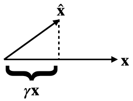
By definition, $\gamma x$ is the multiple of $x$ closest to $\hat{x}$. Equivalently, this closest such vector can be described as the projection ${proj}_x\left(\hat{x}\right)=\frac{\hat{x}\cdot x}{\parallel x{\parallel }_2^2}x$. Setting these equal, we get the... (read more)

Great work! Obviously the results here speak for themselves, but I especially wanted to complement the authors on the writing. I thought this paper was a pleasure to read, and easily a top 5% exemplar of clear technical writing. Thanks for putting in the effort on that.

I'll post a few questions as children to this comment.

I'm pretty sure that you're not correct that the interpretation step from our SHIFT experiments essentially relies on using data from the Pile. I strongly expect that if we were to only use inputs from $D_a$ then we would be able to interpret the SAE features about as well. E.g. some of the SAE features only activate on female pronouns, and we would be able to notice this. Technically, we wouldn't be able to rule out the hypothesis "this feature activates on female pronouns only when their antecedent is a nurse," but that would be a bit of a crazy h... (read more)

(Edits made. In the edited version, I think the only questionable things are the title and the line "[In this post, I will a]rticulate a class of approaches to scalable oversight I call cognition-based oversight." Maybe I should be even more careful and instead say that cognition-based oversight is merely something that "could be useful for scalable oversight," but I overall feel okay about this.

Everywhere else, I think the term "scalable oversight" is now used in the standard way.)

I (mostly; see below) agree that in this post I used the term "scalable oversight" in a way which is non-standard and, moreover, in conflict way the way I typically use the term personally. I also agree with the implicit meta-point that it's important to be careful about using terminology in a consistent way (though I probably don't think it's as important as you do). So overall, after reading this comment, I wish I had been more careful about how I treated the term "scalable oversight." After I post this comment, I'll make some edits for clarity, but I do... (read more)

With the ITO experiments, my first guess would be that reoptimizing the sparse approximation problem is mostly relearning the encoder, but with some extra uninterpretable hacks for low activation levels that happen to improve reconstruction. In other words, I'm guessing that the boost in reconstruction accuracy (and therefore loss recovered) is mostly not due to better recognizing the presence of interpretable features, but by doing fiddly uninterpretable things at low activation levels.

I'm not really sure how to operationalize this into a prediction. Mayb... (read more)

Awesome stuff -- I think that updates like this (both from the GDM team and from Anthropic) are very useful for organizing work in this space. And I especially appreciate the way this was written, with both short summaries and in-depth write-ups.

Yep, as you say, @Logan Riggs figured out what's going on here: you evaluated your reconstruction loss on contexts of length 128, whereas I evaluated on contexts of arbitrary length. When I restrict to context length 128, I'm able to replicate your results.

Here's Logan's plot for one of your dictionaries (not sure which)

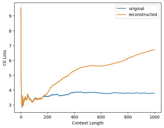
and here's my replication of Logan's plot for your layer 1 dictionary

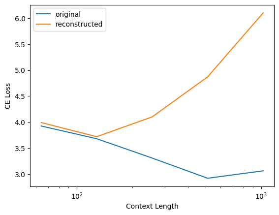
Interestingly, this does not happen for my dictionaries! Here's the same plot but for my layer 1 residual stream output dictionary for pythia-70m-deduped

(Note that all thr... (read more)

My SAEs also have a tied decoder bias which is subtracted from the original activations. Here's the relevant code in dictionary.py

def encode(self, x):
        return nn.ReLU()(self.encoder(x - self.bias))
    
    def decode(self, f):
        return self.decoder(f) + self.bias
    
    def forward(self, x, output_features=False, ghost_mask=None):
            [...]
            f = self.encode(x)
            x_hat = self.decode(f)
            [...]
            return x_hat

Note that I checked that our SAEs have the same input-output behavior in my linked c... (read more)

Another sanity check: when you compute CE loss using the same code that you use when computing CE loss when activations are reconstructed by the autoencoders, but instead of actually using the autoencoder you just plug the correct activations back in, do you get the same answer (~3.3) as when you evaluate CE loss normally?

In the notebook I link in my original comment, I check that the activations I get out of nnsight are the same as the activations that come from transformer_lens. Together with the fact that our sparsity statistics broadly align, I'm guessing that the issue isn't that I'm extracting different activations than you are.

Repeating my replication attempt with data from OpenWebText, I get this:

Broadly speaking, same story as above, e... (read more)

I tried replicating your statistics using my own evaluation code (in evaluation.py here). I pseudo-randomly chose layer 1 and layer 7. Sadly, my results look rather different from yours:

Places where our metrics agree: L1 and L0.

Places where our metrics disagree, but probably for a relatively benign reason:

• Percent variance explained: my numbers are slightly lower than yours, and from a brief skim of your code I think it's bec

Some updates about the dictionary_learning repo:

• The repo now has support for ghost grads. h/t g-w1 for submitting a PR for this
• ActivationBuffers now work natively with model components -- like the residual stream -- whose activations are typically returned as tuples; the buffer knows to take the first component of the tuple (and will iteratively do this if working with nested tuples).
• ActivationBuffers can now be stored on the GPU.
• The file evaluation.py contains code for evaluating trained dictionaries. I've found this pretty useful for quickly evaluating d

Imo "true according to Alice" is nowhere near as "crazy" a feature as "has_true XOR has_banana". It seems useful for the LLM to model what is true according to Alice! (Possibly I'm misunderstanding what you mean by "crazy" here.)

I agree with this! (And it's what I was trying to say; sorry if I was unclear.) My point is that 
{ features which are as crazy as "true according to Alice" (i.e., not too crazy)} 
seems potentially manageable, where as 
{ features which are as crazy as arbitrary boolean functions of other features } 
seems totally unmanageable.

Thanks, as always, for the thoughtful replies.

Idk, I think it's pretty hard to know what things are and aren't useful for predicting the next token. For example, some of your features involve XORing with a "has_not" feature -- XORing with an indicator for "not" might be exactly what you want to do to capture the effect of the "not".

I agree that "the model has learned the algorithm 'always compute XORs with has_not'" is a pretty sensible hypothesis. (And might be useful to know, if true!) FWIW, the stronger example of "clearly not useful XORs" I was thinking of has_true XOR has_banana, where I'm guessi... (read more)

I agree with a lot of this, but some notes:

Exponentially many features

[...]

On utility explanations, you would expect that multi-way XORs are much less useful for getting low loss than two-way XORs, and so computation for multi-way XORs is never developed.

The thing that's confusing here is that the two-way XORs that my experiments are looking at just seem clearly not useful for anything. So I think any utility explanation that's going to be correct needs to be a somewhat subtle one of the form "the model doesn't initially know which XORs will be useful, so ... (read more)

Thanks, you're totally right about the equal variance thing -- I had stupidly thought that the projection of $U\left(\right[0,1{]}^2)$ onto y = x would be uniform on $[-\frac{1}{\sqrt{2}},\frac{1}{\sqrt{2}}]$ (obviously false!).

The case of a fully discrete distribution (supported in this case on four points) seems like a very special case of a something more general, where a "more typical" special case would be something like:

• if a, b are both false, then sample from $N(0,\Sigma )$
• if a is true and b is false, then sample from $N({\mu }_a,\Sigma )$
• if a is false and b is true then sample from 

Thanks, you're correct that my definition breaks in this case. I will say that this situation is a bit pathological for two reasons:

1. The mode of a uniform distribution doesn't coincide with its mean.
2. The variance of the multivariate uniform distribution $U\left(\right[0,1]\times [0,1\left]\right)$ is largest along the direction $x_1+x_2$, which is exactly the direction which we would want to represent a AND b.

I'm not sure exactly which assumptions should be imposed to avoid pathologies like this, but maybe something of the form: we are working with boolean features $f$ ... (read more)

Neat hypothesis! Do you have any ideas for how one would experimentally test this?

Some features which are computed from other features should probably themselves be treated as basic and thus represented with large salience.

Using a dataset of 10,000 inputs of the form
[random LLaMA-13B generated text at temperature 0.8] [either the most likely next token or the 100th most likely next token, according to LLaMA-13B] ["true" or "false"] ["banana" or "shed"]
I've rerun the probing experiments. The possible labels are

• has_true: is the second last token "true" or "false"?
• has_banana: is the last token "banana" or "shed"?
• label: is the third last token the most likely or the 100th most likely?

(this weird last option is because I'm adapting a dataset from the Geometry of Truth paper about... (read more)

Yes, you are correct, thanks. I'll edit the post when I get a chance.

If anyone would like to replicate these results, the code can be found in the rax branch of my geometry-of-truth repo. This was adapted from a codebase I used on a different project, so there's a lot of uneeded stuff in this repo. The important parts here are:

• The datasets: cities_alice.csv and neg_cities_alice.csv (for the main experiments I describe), cities_distractor.csv and neg_cities_distractor.csv (for the experiments with banana/shed at the end of factual statements), and xor.csv (for the experiments with true/false and banana/shed after random text

Thanks for doing this! Can you share the dataset that you're working with? I'm traveling right now, but when I get a chance I might try to replicate your failed replication on LLaMA-2-13B and with my codebase (which can be found here; see especially xor_probing.ipynb).

Idk, I think I would guess that all of the most salient features will be things related to the meaning of the statement at a more basic level. E.g. things like: the statement is finished (i.e. isn't an ongoing sentence), the statement is in English, the statement ends in a word which is the name of a country, etc.

My intuition here is mostly based on looking at lots of max activating dataset examples for SAE features for smaller models (many of which relate to basic semantic categories for words or to basic syntax), so it could be bad here (both because of ... (read more)

There's 1500 statements in each of cities and neg_cities, and LLaMA-2-13B has residual stream dimension 5120. The linear probes are trained with vanilla logistic regression on {80% of the data in cities} \cup {80% of the data in neg_cities} and the accuracies reported are evaluated on {remaining 20% of the data in cities} \cup {remaining 20% of the data in neg_cities}.

So, yeah, I guess that the train and val sets are drawn from the same distribution but are not independent (because of the issue I mentioned in my comment above). Oops! I guess I never though... (read more)

(Are you saying that you think factuality is one of the 50 most salient features when the model processes inputs like "The city of Chicago is not in Madagascar."? I think I'd be pretty surprised by this.)

(To be clear, factuality is one of the most salient feature relative to the cities/neg_cities datasets, but it seems like the right notion of salience here is relative to the full data distribution.)

I'm not really sure, but I don't think this is that surprising. I think when we try to fit a probe to "label" (the truth value of the statement), this is probably like fitting a linear probe to random data. It might overfit on some token-level heuristic which is ideosyncratically good on the train set but generalizes poorly to the val set. E.g. if disproportionately many statements containing "India" are true on the train set, then it might learn to label statements containing "India" as true; but since in the full dataset, there is no correlation between "India" and being true, correlation between "India" and true in the val set will necessarily have the opposite sign.

The thing that remains confusing here is that for arbitrary features like these, it's not obvious why the model is computing any nontrivial boolean function of them and storing it along a different direction. And if the answer is "the model computes this boolean function of arbitrary features" then the downstream consequences are the same, I think.

What is "this"? It sounds like you're gesturing at the same thing I discuss in the section "Maybe $a\oplus b$ is represented “incidentally” because it’s possible to aggregate noisy signals from many features which are correlated with boolean functions of a and b"

Thanks! I'm still pretty confused though.

It sounds like you're making an empirical claim that in this banana/shed example, the model is representing the features $\text{has\_banana}\left(x\right)$, $\text{has\_true}\left(x\right)$, and $\text{has\_banana}\left(x\right)\oplus \text{has\_true}\left(x\right)$ along linearly independent directions. Are you saying that this claim is supported by PCA visualizations you've done? Maybe I'm missing something, but none of the PCA visualizations I'm seeing in the paper seem to touch on this. E.g. visualization in figure 2(b) (reproduced below) is colored by $\text{is\_true}\left(x\right)$, not ... (read more)