High-speed intro to Bayes's rule
(This is a high-speed introduction to Bayes' rule for people who want to get straight to it and are good at math. If you'd like a gentler or more thorough introduction, try starting at the Bayes' Rule Guide page instead.)
Percentages, frequencies, and waterfalls
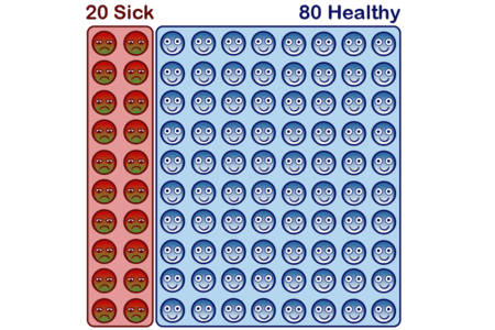
Suppose you're screening a set of patients for a disease, which we'll call Diseasitis.[1] Your initial test is a tongue depressor containing a chemical strip, which usually turns black if the patient has Diseasitis.
- Based on prior epidemiology, you expect that around 20% of patients in the screening population have Diseasitis.
- Among patients with Diseasitis, 90% turn the tongue depressor black.
- 30% of the patients without Diseasitis will also turn the tongue depressor black.
What fraction of patients with black tongue depressors have Diseasitis?
Answer
3/7 or 43%, quickly obtainable as follows: In the screened population, there's 1 sick patient for 4 healthy patients. Sick patients are 3 times more likely to turn the tongue depressor black than healthy patients. or 3 sick patients to 4 healthy patients among those that turn the tongue depressor black, corresponding to a probability of that the patient is sick.
(Take your own stab at answering this question, then please click "Answer" above to read the answer before continuing.)
Bayes' rule is a theorem which describes the general form of the operation we carried out to find the answer above. In the form we used above, we:
- Started from the prior odds of (1 : 4) for sick versus healthy patients;
- Multiplied by the likelihood ratio of (3 : 1) for sick versus healthy patients blackening the tongue depressor;
- Arrived at posterior odds of (3 : 4) for a patient with a positive test result being sick versus healthy.
Bayes' rule in this form thus states that the prior odds times the likelihood ratio equals the posterior odds.
We could also potentially see the positive test result as revising a prior belief or prior probability of 20% that the patient was sick, to a posterior belief or posterior probability of 43%.
To make it clearer that we did the correct calculation above, and further pump intuitions for Bayes' rule, we'll walk through some additional visualizations.
Frequency representation
The frequency representation of Bayes' rule would describe the problem as follows: "Among 100 patients, there will be 20 sick patients and 80 healthy patients."
"18 out of 20 sick patients will turn the tongue depressor black. 24 out of 80 healthy patients will blacken the tongue depressor."
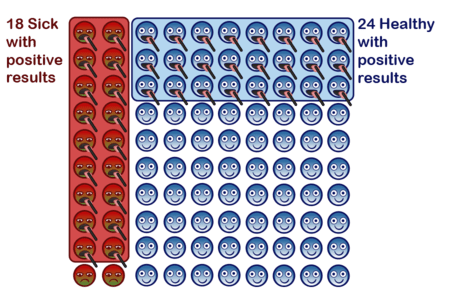
"Therefore, there are (18+24)=42 patients who turn the tongue depressor black, among whom 18 are actually sick. (18/42)=(3/7)=43%."
(Some experiments show [2] that this way of explaining the problem is the easiest for e.g. medical students to understand, so you may want to remember this format for future use. Assuming you can't just send them to Arbital!)
Waterfall representation
The waterfall representation may make clearer why we're also allowed to transform the problem into prior odds and a likelihood ratio, and multiply (1 : 4) by (3 : 1) to get posterior odds of (3 : 4) and a probability of 3/7.
The following problem is isomorphic to the Diseasitis one:
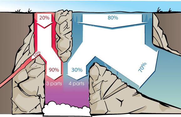
"A waterfall has two streams of water at the top, a red stream and a blue stream. These streams flow down the waterfall, with some of each stream being diverted off to the side, and the remainder pools at the bottom of the waterfall."
"At the top of the waterfall, there's around 20 gallons/second flowing from the red stream, and 80 gallons/second flowing from the blue stream. 90% of the red water makes it to the bottom of the waterfall, and 30% of the blue water makes it to the bottom of the waterfall. Of the purplish water that mixes at the bottom, what fraction is from the red stream versus the blue stream?"
We can see from staring at the diagram that the prior odds and likelihood ratio are the only numbers we need to arrive at the answer:
- The problem would have the same answer if there were 40 gallons/sec of red water and 160 gallons/sec of blue water (instead of 20 gallons/sec and 80 gallons/sec). This would just multiply the total amount of water by a factor of 2, without changing the ratio of red to blue at the bottom.
- The problem would also have the same answer if 45% of the red stream and 15% of the blue stream made it to the bottom (instead of 90% and 30%). This would just cut down the total amount of water by a factor of 2, without changing the relative proportions of red and blue water.
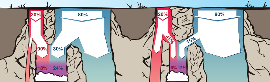
So only the ratio of red to blue water at the top (prior odds of the proposition), and only the ratio between the percentages of red and blue water that make it to the bottom (likelihood ratio of the evidence), together determine the posterior ratio at the bottom: 3 parts red to 4 parts blue.
Test problem
Here's another Bayesian problem to attempt. If you successfully solved the earlier problem on your first try, you might try doing this one in your head.
10% of widgets are bad and 90% are good. 4% of good widgets emit sparks, and 12% of bad widgets emit sparks. What percentage of sparking widgets are bad?
Answer
- There's bad vs. good widgets. (9 times as many good widgets as bad widgets; widgets are 1/9 as likely to be bad as good.)
- Bad vs. good widgets have a relative likelihood to spark, which simplifies to (Bad widgets are 3 times as likely to emit sparks as good widgets.)
- (1 bad sparking widget for every 3 good sparking widgets.)
- Odds of convert to a probability of (25% of sparking widgets are bad.)
(If you're having trouble using odds ratios to represent uncertainty, see this intro or this page.)
General equation and proof
To say exactly what we're doing and prove its validity, we need to introduce some notation from probability theory.
If is a proposition, will denote 's probability, our quantitative degree of belief in
will denote the negation of or the proposition " is false".
If and are propositions, then denotes the proposition that both X and Y are true. Thus denotes "The probability that and are both true."
We now define conditional probability:
We pronounce as "the conditional probability of X, given Y". Intuitively, this is supposed to mean "The probability that is true, assuming that proposition is true".
Defining conditional probability in this way means that to get "the probability that a patient is sick, given that they turned the tongue depressor black" we should put all the sick plus healthy patients with positive test results into a bag, and ask about the probability of drawing a patient who is sick and got a positive test result from that bag. In other words, we perform the calculation
Rearranging the definition of conditional probability, So to find "the fraction of all patients that are sick and get a positive result", we multiply "the fraction of patients that turn the tongue depressor black" times "the probability that a sick patient blackens the tongue depressor".
We're now ready to prove Bayes's rule in the form, "the prior odds times the likelihood ratio equals the posterior odds".
The "prior odds" is the ratio of sick to healthy patients:
The "likelihood ratio" is how much more relatively likely a sick patient is to get a positive test result (turn the tongue depressor black), compared to a healthy patient:
The "posterior odds" is the odds that a patient is sick versus healthy, given that they got a positive test result:
Bayes's theorem asserts that prior odds times likelihood ratio equals posterior odds:
We will show this by proving the general form of Bayes's Rule. For any two hypotheses and and any piece of new evidence :
In the Diseasitis example, this corresponds to performing the operations:
Using red for sick, blue for healthy, grey for a mix of sick and healthy patients, and + signs for positive test results, the proof above can be visualized as follows:
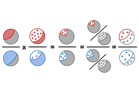
less red in first circle (top left). in general, don't have prior proportions equal posterior proportions graphically!
Bayes' theorem
An alternative form, sometimes called "Bayes' theorem" to distinguish it from "Bayes' rule" (although not everyone follows this convention), uses absolute probabilities instead of ratios. The law of marginal probability states that for any set of mutually exclusive and exhaustive possibilities and any proposition :
Then we can derive an expression for the absolute (non-relative) probability of a proposition after observing evidence as follows:
The equation of the first and last terms above is what you will usually see described as Bayes' theorem.
To see why this decomposition might be useful, note that is an inferential step, a conclusion that we make after observing a new piece of evidence. is a piece of causal information we are likely to have on hand, for example by testing groups of sick patients to see how many of them turn the tongue depressor black. describes our state of belief before making any new observations. So Bayes' theorem can be seen as taking what we already believe about the world (including our prior belief about how different imaginable states of affairs would generate different observations), plus an actual observation, and outputting a new state of belief about the world.
Vector and functional generalizations
Since the proof of Bayes' rule holds for any pair of hypotheses, it also holds for relative belief in any number of hypotheses. Furthermore, we can repeatedly multiply by likelihood ratios to chain together any number of pieces of evidence.
Suppose there's a bathtub full of coins:
- Half the coins are "fair" and have a 50% probability of coming up Heads each time they are thrown.
- A third of the coins are biased to produce Heads 25% of the time (Tails 75%).
- The remaining sixth of the coins are biased to produce Heads 75% of the time.
You randomly draw a coin, flip it three times, and get the result HTH. What's the chance this is a fair coin?
We can validly calculate the answer as follows:
So the posterior probability the coin is fair is 8/13 or ~62%.
This is one reason it's good to know the odds form of Bayes' rule, not just the probability form in which Bayes' theorem is often given.[3]
We can generalize further by writing Bayes' rule in a functional form. If is a relative belief vector or relative belief function on the variable and is the likelihood function giving the relative chance of observing evidence given each possible state of affairs then relative posterior belief is given by:
If we normalize the relative odds into absolute probabilities - that is, divide through by its sum or integral so that the new function sums or integrates to - then we obtain Bayes' rule for probability functions:
Applications of Bayesian reasoning
This general Bayesian framework - prior belief, evidence, posterior belief - is a lens through which we can view a lot of formal and informal reasoning plus a large amount of entirely nonverbal cognitive-ish phenomena.[4]
Examples of people who might want to study Bayesian reasoning include:
- Professionals who use statistics, such as scientists or medical doctors.
- Computer programmers working in the field of machine learning.
- Human beings trying to think.
The third application is probably of the widest general interest.
Example human applications of Bayesian reasoning
Philip Tetlock found when studying "superforecasters", people who were especially good at predicting future events:
"The superforecasters are a numerate bunch: many know about Bayes' theorem and could deploy it if they felt it was worth the trouble. But they rarely crunch the numbers so explicitly. What matters far more to the superforecasters than Bayes' theorem is Bayes' core insight of gradually getting closer to the truth by constantly updating in proportion to the weight of the evidence." — Philip Tetlock and Dan Gardner, Superforecasting
This is some evidence that knowing about Bayes' rule and understanding its qualitative implications is a factor in delivering better-than-average intuitive human reasoning. This pattern is illustrated in the next couple of examples.
The OKCupid date.
One realistic example of Bayesian reasoning was deployed by one of the early test volunteers for a much earlier version of a guide to Bayes' rule. She had scheduled a date with a 96% OKCupid match, who had then cancelled that date without other explanation. After spending some mental time bouncing back and forth between "that doesn't seem like a good sign" versus "maybe there was a good reason he canceled", she decided to try looking at the problem using that Bayes thing she'd just learned about. She estimated:
- A 96% OKCupid match like this one, had prior odds of 2 : 5 for being a desirable versus undesirable date. (Based on her prior experience with 96% OKCupid matches, and the details of his profile.)
- Men she doesn't want to go out with are 3 times as likely as men she might want to go out with to cancel a first date without other explanation.
This implied posterior odds of 2 : 15 that this was an undesirable date, which was unfavorable enough not to pursue him further.[5]
The point of looking at the problem this way is not that she knew exact probabilities and could calculate that the man had an exactly 88% chance of being undesirable. Rather, by breaking up the problem in that way, she was able to summarize what she thought she knew in compact form, see what those beliefs already implied, and stop bouncing back and forth between imagined reasons why a good date might cancel versus reasons to protect herself from potential bad dates. An answer roughly in the range of 15/17 made the decision clear.
Internment of Japanese-Americans during World War II
From Robyn Dawes's Rational Choice in an Uncertain World:
Post-hoc fitting of evidence to hypothesis was involved in a most grievous chapter in United States history: the internment of Japanese-Americans at the beginning of the Second World War. When California governor Earl Warren testified before a congressional hearing in San Francisco on February 21, 1942, a questioner pointed out that there had been no sabotage or any other type of espionage by the Japanese-Americans up to that time. Warren responded, "I take the view that this lack subversive activity is the most ominous sign in our whole situation. It convinces me more than perhaps any other factor that the sabotage we are to get, the Fifth Column activities are to get, are timed just like Pearl Harbor was timed... I believe we are just being lulled into a false sense of security."
You might want to take your own shot at guessing what Dawes had to say about a Bayesian view of this situation, before reading further.
Answer
Suppose we put ourselves into the shoes of this congressional hearing, and imagine ourselves trying to set up this problem.
- The prior odds that there would be a conspiracy of Japanese-American saboteurs.
- The likelihood of the observation "no visible sabotage or any other type of espionage", given that a Fifth Column actually existed.
- The likelihood of the observation "no visible sabotage from Japanese-Americans", in the possible world where there is no such conspiracy.
As soon as we set up this problem, we realize that, whatever the probability of "no sabotage" being observed if there is a conspiracy, the likelihood of observing "no sabotage" if there isn't a conspiracy must be even higher. This means that the likelihood ratio:
...must be less than 1, and accordingly:
Observing the total absence of any sabotage can only decrease our estimate that there's a Japanese-American Fifth Column, not increase it. (It definitely shouldn't be "the most ominous" sign that convinces us "more than any other factor" that the Fifth Column exists.)
Again, what matters is not the exact likelihood of observing no sabotage given that a Fifth Column actually exists. As soon as we set up the Bayesian problem, we can see there's something qualitatively wrong with Earl Warren's reasoning.
Further reading
This has been a very brief and high-speed presentation of Bayes and Bayesianism. It should go without saying that a vast literature, nay, a universe of literature, exists on Bayesian statistical methods and Bayesian epistemology and Bayesian algorithms in machine learning. Staying inside Arbital, you might be interested in moving on to read:
More on the technical side of Bayes' rule
- A sadly short list of example Bayesian word problems. Want to add more? (Hint hint.)
- Bayes' rule: Proportional form. The fastest way to present a step in Bayesian reasoning in a way that will sound sort of understandable to somebody who's never heard of Bayes.
- Bayes' rule: Log-odds form. A simple transformation of Bayes' rule reveals tools for measuring degree of belief, and strength of evidence.
- The "Naive Bayes" algorithm. (Scroll down to the middle.) The original simple Bayesian spam filter.
- Non-naive multiple updates. (Scroll down past Naive Bayes.) How to avoid double-counting the evidence, or worse, when considering multiple items of correlated evidence.
- Laplace's Rule of Succession. The classic example of an inductive prior.
More on intuitive implications of Bayes' rule
- A Bayesian view of scientific virtues. Why is it that science relies on bold, precise, and falsifiable predictions? Because of Bayes' rule, of course.
- Update by inches. It's virtuous to change your mind in response to overwhelming evidence. It's even more virtuous to shift your beliefs a little bit at a time, in response to all evidence (no matter how small).
- Belief revision as probability elimination. Update your beliefs by throwing away large chunks of probability mass.
- Shift towards the hypothesis of least surprise. When you see new evidence, ask: which hypothesis is least surprised?
- Extraordinary claims require extraordinary evidence. The people who adamantly claim they were abducted by aliens do provide some evidence for aliens. They just don't provide quantitatively enough evidence.
- Ideal reasoning via Bayes' rule. Bayes' rule is to reasoning as the Carnot cycle is to engines: Nobody can be a perfect Bayesian, but Bayesian reasoning is still the theoretical ideal.
- Likelihoods, p-values, and the replication crisis. Arguably, a large part of the replication crisis can ultimately be traced back to the way journals treat p-values, and a large number of those problems can be summed up as "P-values are not Bayesian."
- ^︎
Lit. "inflammation of the disease".
- ^︎
E.g. "Probabilistic reasoning in clinical medicine" by David M. Eddy (1982).
- ^︎
Imagine trying to do the above calculation by repeatedly applying the form of the theorem that says:
- ^︎
This broad statement is widely agreed. Exactly which phenomena are good to view through a Bayesian lens is sometimes disputed.
- ^︎
She sent him what might very well have been the first explicitly Bayesian rejection notice in dating history, reasoning that if he wrote back with a Bayesian counterargument, this would promote him to being interesting again. He didn't write back.