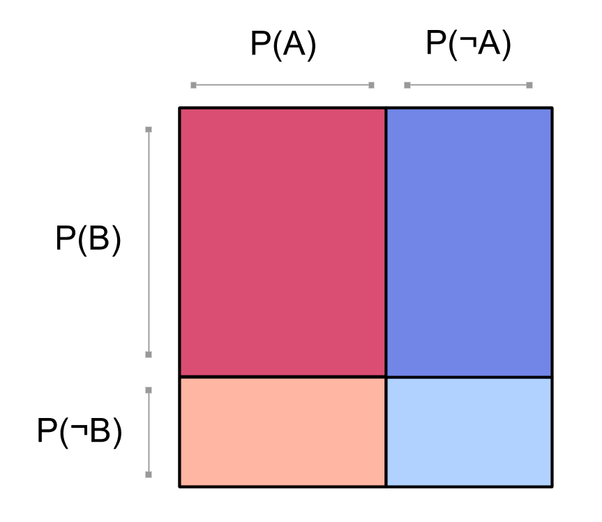
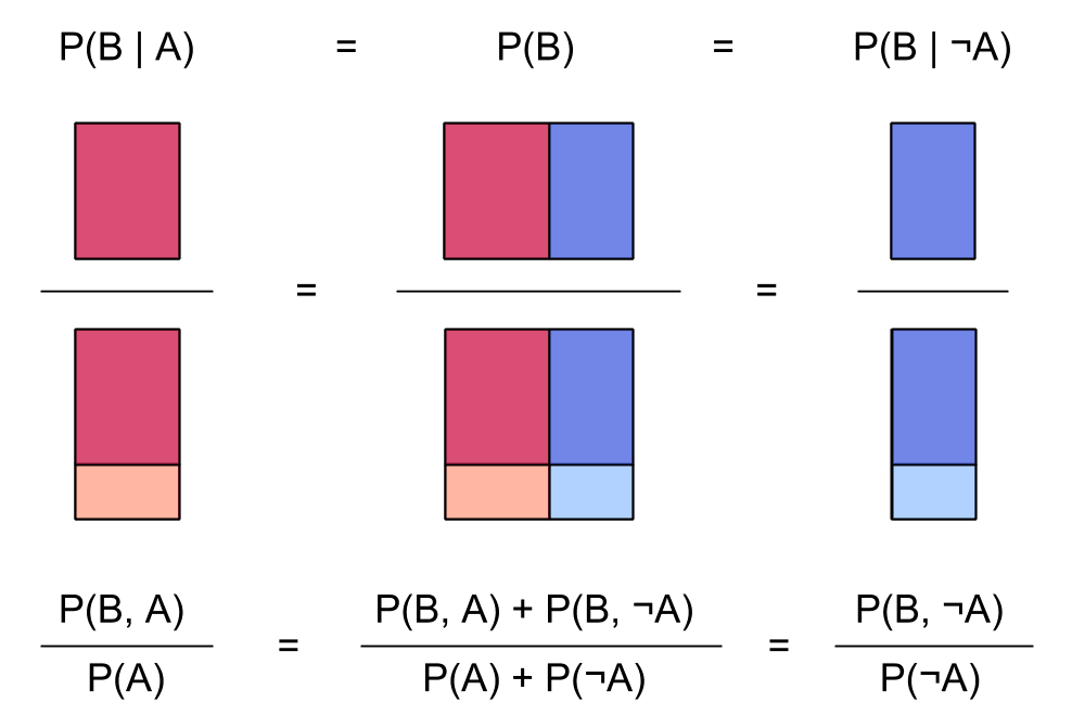
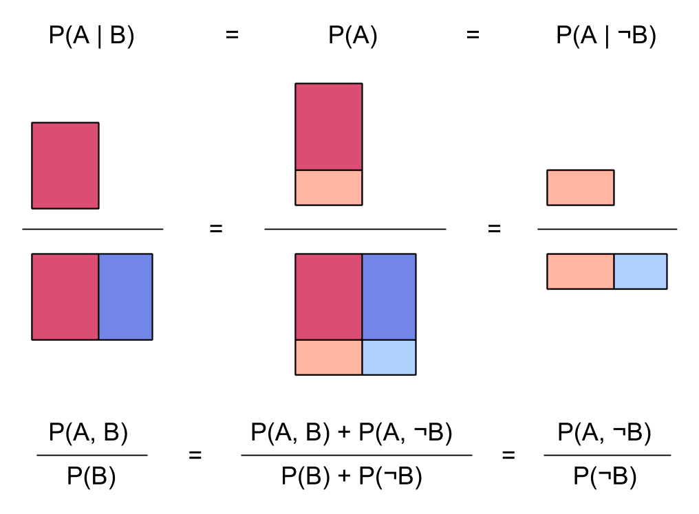
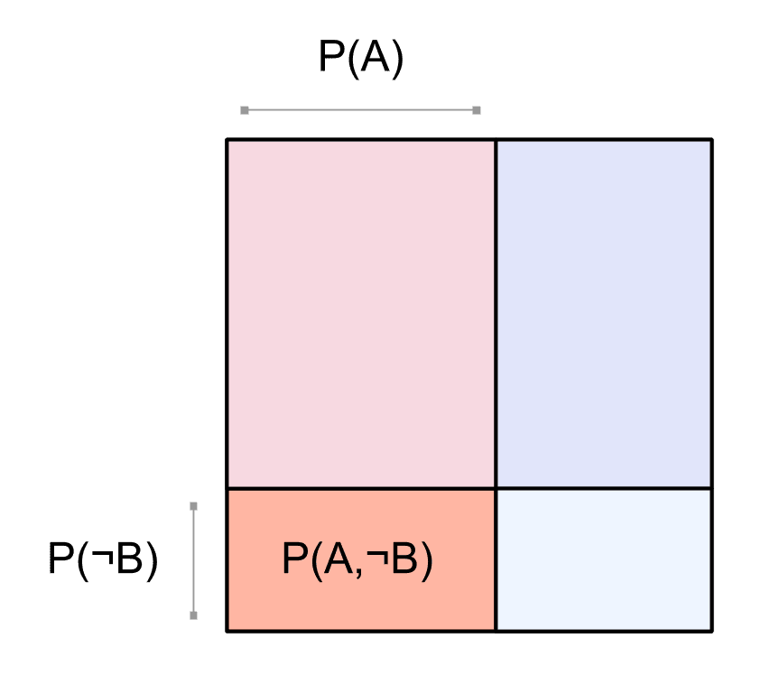
This is what independence looks like, using the square visualization of probabilities:
We can see that the events and don't interact; we say that and are independent. Whether we look at the whole square, or just the red part of the square where is true, the probability of stays the same. In other words, . That's what we mean by independence: the probability of doesn't change if you condition on .
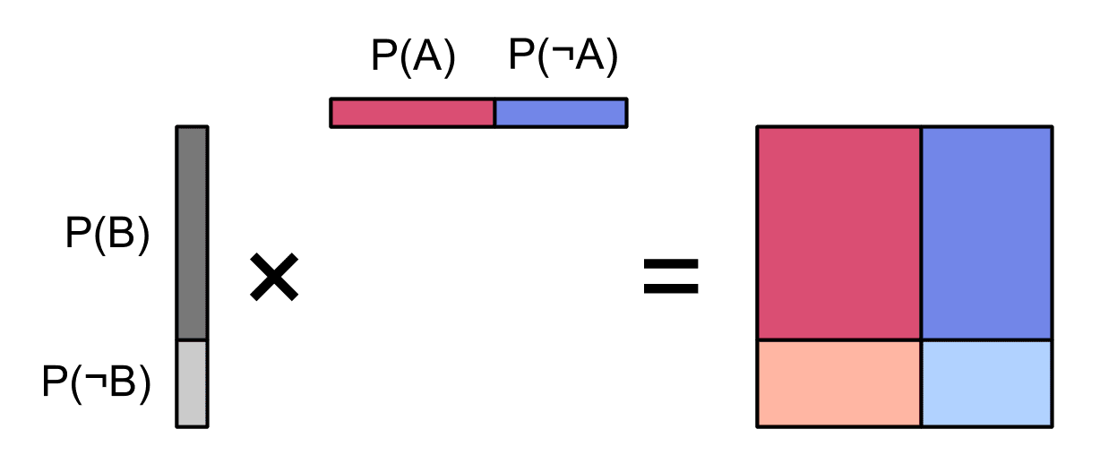
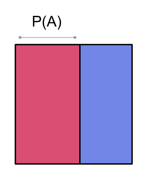
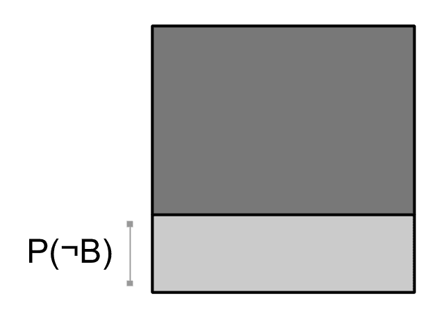
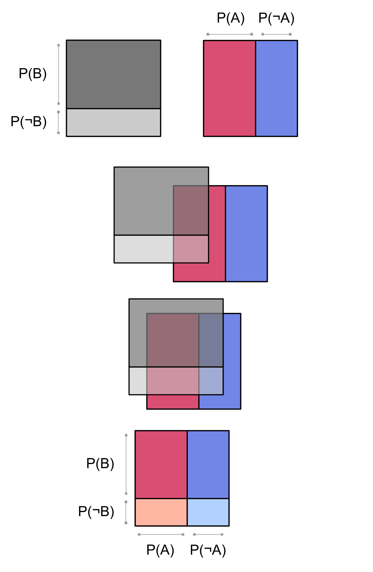
Our square of probabilities can be generated by multiplying together the probability of and the probability of :
This picture demonstrates another way to define what it means for and to be independent:
In terms of factoring a joint distribution --
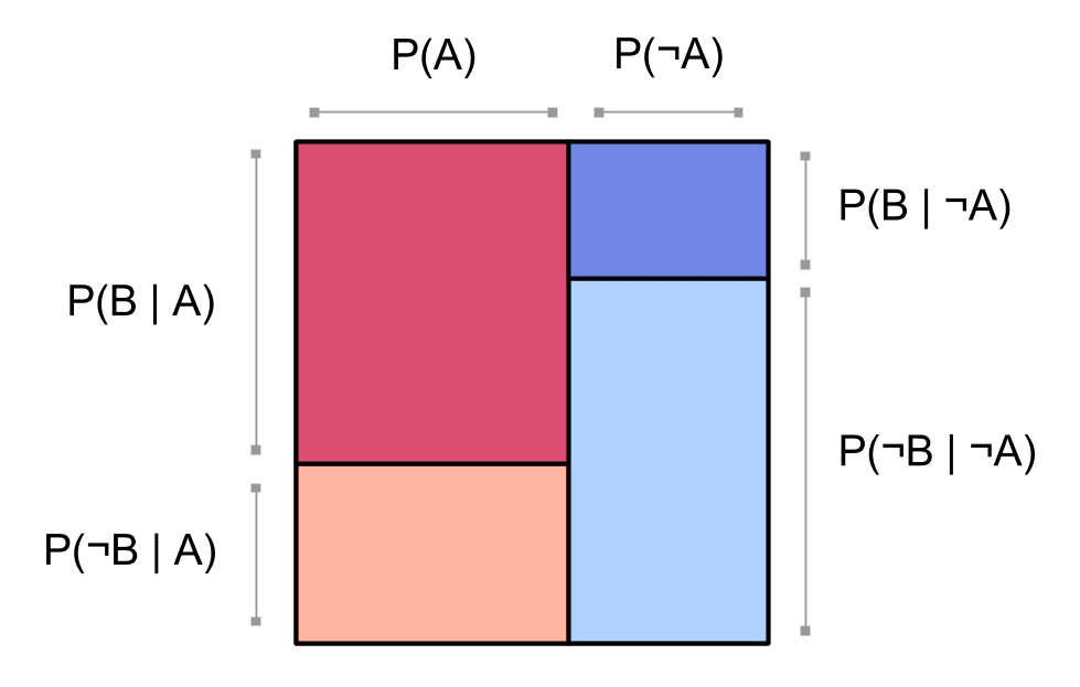
Let's contrast independence with non-independence. Here's a picture of two ordinary, non-independent events and :
(If the meaning of this picture isn't clear, take a look at Square visualization of probabilities on two events.)
We have the red blocks for and the blue blocks for lined up in columns. This means we've factored our probability distribution using as the first factor:
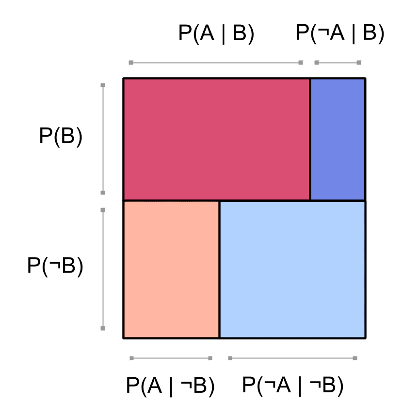
We could just as well have factored by first: Then we'd draw a picture like this:
Now, here again is the picture of two independent events and :
In this picture, there's red and blue lined-up columns for and , and there's also dark and light lined-up rows for and . It looks like we somehow factored our probability distribution using both and as the first factor.
In fact, this is exactly what happened: since and are independent, we have that . So the diagram above is actually factored according to first: . It's just that , since is independent from . So we don't need to have different ratios of dark to light (a.k.a. conditional probabilities of ) in the left and right columns:
In this visualization, we can see what happens to the probability of when you condition on or on : it doesn't change at all. The ratio of [the area where happens] to [the whole area], is the same as the ratio where we only look at the area where happens, which is the same as the ratio where we only look at the area where happens. The fact that the probability of doesn't change when we condition on is exactly what we mean when we say that and are independent.
The square diagram above is also factored according to first, using . The red / blue ratios are the same in both rows because , since and are independent:
We couldn't do any of this stuff if the columns and rows didn't both line up. (Which is good, because then we'd have proved the false statement that any two events are independent!)
In terms of multiplying marginal probabilities
Another way to say that and are independent variables [1] is that for any truth values
So the joint probabilities for and are computed by separately getting the probability of and the probability of , and then multiplying the two probabilities together. For example, say we want to compute the probability . We start with the marginal probability of :
and the probability of :
and then we multiply them:
We can get all the joint probabilities this way. So we can visualize the whole joint distribution as the thing that you get when you multiply two independent probability distributions together. We just overlay the two distributions:
To be a little more mathematically elegant, we'd use the topological product of two spaces shown earlier to draw the joint distribution as a product of the distributions of and :
- ^︎
We're using the equivalence between [event_probability events] and binary variables.
