This post is the result of a 2 week research sprint project during the training phase of Neel Nanda’s MATS stream. 

Executive Summary

• We replicate Anthropic's MLP Sparse Autoencoder (SAE) paper on attention outputs and it works well: the SAEs learn sparse, interpretable features, which gives us insight into what attention layers learn. We study the second attention layer of a two layer language model (with MLPs).
  • Specifically, rather than training our SAE on attn_output, we train our SAE on “hook_z” concatenated over all attention heads (aka the mixed values aka the attention outputs before a linear map - see notation here). This is valuable as we can see how much of each feature’s weights come from each head, which we believe is a promising direction to investigate attention head superposition, although we only briefly explore that in this work.
• We open source our SAE, you can use it via this Colab notebook.
• Shallow Dives: We do a shallow investigation to interpret each of the first 50 features. We estimate 82% of non-dead features in our SAE are interpretable (24% of the SAE features are dead).
  • See this feature interface to browse the first 50 features.
• Deep dives: To verify our SAEs have learned something real, we zoom in on individual features for much more detailed investigations: the  “‘board’ is next by induction” feature, the local context feature of “in questions starting with ‘Which’”, and the more global context feature of “in texts about pets”.
  • We go beyond the techniques from the Anthropic paper, and investigate the circuits used to compute the features from earlier components, including analysing composition with an MLP0 SAE. 
  • We also investigate how the features are used downstream, and whether it's via MLP1 or the direct connection to the logits. 
• Automation: We automatically detect and quantify a large “{token} is next by induction” feature family. This represents ~5% of the living features in the SAE.
  • Though the specific automation technique won't generalize to other feature families, this is notable, as if there are many “one feature per vocab token” families like this, we may need impractically wide SAEs for larger models.

Introduction

In Anthropic’s SAE paper, they find that training sparse autoencoders (SAEs) on a one layer model’s MLP activations finds interpretable features, providing a path to breakdown these high dimensional activations into units that we can understand. In this post, we demonstrate that the same technique works on attention layer outputs and learns sparse, interpretable features! 

To see how interpretable our SAE is we perform shallow investigations of the first 50 features of our SAE (i.e. randomly chosen features). We found that 76% are not dead (i.e. activate on at least some inputs), and within the alive features we think 82% are interpretable. To get a feel for the features we find see our interactive visualizations of the first 50. Here’s one example:^[1]

Shallow investigations are limited and may be misleading or illusory, so we then do some deep dives to more deeply understand multiple individual features including:

• “‘board’ is next, by induction” - one of many “{token} is next by induction" features
• “In questions starting with ‘Which’” - a local context feature, which interestingly is computed by multiple heads
• “In pet context” - one of many high level context features

Similar to the Anthropic paper’s “Detailed Investigations”, we understand when these features activate and how they affect downstream computation. However, we also go beyond Anthropic’s techniques, and look into the upstream circuits by which these features are computed from earlier components. An attention layer (with frozen attention pattern) is a linear function of earlier residual streams, so unlike MLP layers it's easy to step backwards through the model and see where these features come from.

Leveraging insights from our induction feature case study, we also use heuristics to automatically identify and quantify a large feature family of the form: “{token} is next by induction”. Interestingly, this is a feature family that we expect to be unique to attention outputs. It also suggests that we should have a feature per token, implying that the SAE needs to be at least ~50k features wide. If there are many families with per token features, naively training an SAE to extract every feature may be extremely expensive. 

Our SAE

Our SAE was trained on the attention outputs from the final layer of gelu-2l. Specifically, we train our SAE on the “z” vectors concatenated across all heads of the last layer. Note that “z” is the weighted sum of “values” before they are converted to the attention output by a linear map. See this diagram, from Callum McDougall’s ARENA, for reference on the different activations within a transformer attention layer (using TransformerLens notation):

 (Alternatively, the z value is covered in Neel’s transformer tutorial and can be found here in TransformerLens.)

We see “z” vs “attn_out” as basically a technicality, as z is a linear transformation of attn_out since there's just a linear map between them, and thus we expect to find the same features. However, we deliberately trained our SAE on “z” since we find that this helps us attribute which heads the weights and activations are from for each SAE feature. To be clear, we are not training on the “q”, “k”, “v”, “attn patterns”, “result” or “attn_out” activations. We are also not training on the “z” vectors for a specific head, but instead concatenate all the “z” vectors over all heads in L1.

The important hyperparameters / training details include:

• Width of 16384 features (32x wider than the concatenated z size of 512)
• L1 coefficient: 2
• Learning rate: 1e-3
• Batch size: 4096
• Neuron resampling scheme: at training steps 50000, 100000, 150000, and 200000 we identify features that fired with log frequency less than 1e-7 in the last 25000 steps, and reinitialize their encoder and decoder weights using a Kaiming Uniform initialization. We also reset the Adam optimizer parameters for every modified weight and bias term.
• Trained on 2B tokens of 80% c4 (web text) and 20% code
• Trained on a single A6000 (48 GB) overnight
• See our wandb dashboards for more, including feature density histograms

Our resulting SAE had an average L0 norm of ~12 with ~87% loss recovered, and ~24% dead features. It’s worth noting that we didn’t do anything fancy or iterate on this a ton, yet it still worked quite well. We’re pretty optimistic that we could get even cleaner results with simple improvements like increasing the autoencoder width and implementing Anthropic’s resampling scheme.

Feature Deep Dives

Similar to Anthropic’s “Detailed Investigations of Individual Features”, we perform deep dives on multiple features from our SAE. For each feature, we try to rigorously study the following questions:

1. In what context does the feature activate?
2. How does the feature affect downstream computation?
3. How is the feature computed by upstream components?

We look at examples from three feature families: induction features ("board" is next by induction), local context features (in a question starting with "which") and high-level context features (in a text related to pets). In the interests of brevity, we give a detailed analysis of the first feature, and for the second and third features we relegated much of the analysis with analogous techniques to the appendix, and focus in the main text on what's novel about the other feature families.

Induction Feature: Board induction

We used our SAE to extract and understand a “‘board’ is next by induction” feature. We were excited to find this feature because it seems to be unique to attention, as we are not aware of any induction features in MLP SAEs. It’s also one of many “{token} is next by induction” features, a feature family which we investigate more in the automated induction feature section.

From our shallow investigations we noticed:

1. It fires on repeated tokens
2. The top logit contribution is “board”
3. The norm for the decoder weights corresponding to head 1.6, an induction head, is relatively large

Thus we hypothesize is that this feature activates on the second instance of <token> in prompts of the form “<token> board … <token>”.

Specificity / Sensitivity Analysis

Our first step is to check that the activation of this feature is specific to this context. We created a proxy that checks for cases of strict “board” induction (and some instances of fuzzy induction) and compared the activation of our proxy to the activation of the feature:

While the upper parts of the activation spectrum clearly respond with high specificity to ‘board’ induction, there are plenty of false positives in the lower activation ranges. We suspect that there are two main explanations for this:

• Our proxy is imperfect. Manually staring at the false positives in the medium activation ranges reveals examples of fuzzy ‘board’ induction that weren’t identified by our simple proxy: 

• Our autoencoder is too small: the SAE only has a width of ~16,000. We expect our model to have many more “true features” (note there are 50k tokens in the vocabulary). Thus unrecovered features may show up as linear combinations of many of our learned features

We also agree with the following intuition from the Anthropic paper: “large feature activations have larger impacts on model predictions, so getting their interpretation right matters most”. Thus we reproduce their expected value plots to demonstrate that most of the magnitude of activation provided by this feature comes from ‘board’ induction examples.

We now analyze activation sensitivity. We found 68 false negatives in a dataset of 1 million tokens and manually checked them. We find that while they technically satisfy the ‘board’ induction pattern, it’s pretty clear that ‘board’ should not be predicted.

We also find a Pearson correlation of 0.50 between the activity of our feature and the activity of the proxy over a dataset of 1 million tokens.^[2]

Analyzing Downstream Effects

We now demonstrate that the presence of this feature has an interpretable causal effect on the outputs. We claim this feature is mostly used to predict the “board” token.

We start by analyzing the direct logit effect. We clearly see that the “board” token is the top logit:

We also ablate the feature and observe how this affects per token loss. We find that 82% of total loss increase is explained by tokens where board is the correct next token:

There are two ways the attention layer can affect the loss, by composing with the MLP in Layer 1, and by directly affecting the logits (the direct path term). We perform path patching experiments to investigate this. We find that the direct path is more important to understand than the composition with MLP1, as loss increases when just ablating the feature’s path to mlp_in are both less frequent and lower in magnitude compared to when ablating the feature’s direct path to the logits:

Our path patching experiments also confirm that the feature’s direct effect is mostly predicting ‘board’, as 84% of the total loss increase when ablating the direct path is explained by “board” predictions. For mlp_in, 55% is explained by board predictions. We did not study the composition with the MLP in more detail, although this may be an interesting area of future work.

Understanding how the feature is computed 

Exploiting the idea that attention layers are extremely linear, we go beyond the Anthropic paper to study how upstream components compute this feature.

We first want to investigate what attention heads are used to compute this feature. Since the feature activation is just the dot product (plus encoder bias) of the concatenated z vector and the corresponding column of the encoder matrix, we can rewrite this as the sum of n_heads dot products, allowing us to look at the direct contribution from each head. We call this “direct feature attribution” (as it’s analogous to direct logit attribution), or DFA. We find that head 1.6 dominates with 94% fraction of variance explained^[3] (over the entire dataset)

We confirm that this is an induction head by checking the attention patterns on sequences of repeated random tokens. (Independently corroborated by the Induction Mosaic)

Given that attention heads move information between positions, we also want to learn what information head 1.6 is using to compute this feature. Since the “z” vector is just a weighted sum of the “value” vectors at each source position, we can apply the same direct feature attribution idea to determine which source positions are being moved by head 1.6 to compute this feature. We find that “board” source tokens stand out, suggesting that 1.6 is copying board tokens to compute this feature.

To quantify this we apply DFA by source position for head 1.6 over the entire dataset, and find that the majority of variance is explained by “board” source tokens. This effect gets stronger if we filter for activations above a certain threshold, reaching over 99.9% at a threshold of 5, mirroring Bricken et al's results that there's more polysemanticity in lower ranges.

Attn pattern analysis: convinced that 1.6 is mostly moving “board” token information to compute the feature, we expect to see that it also attends to these tokens. We confirm that when the feature is active, 1.6 mostly attends to “board” tokens

Finally, we go even further upstream and try to localize what components in layer 0 are used to compute this feature. We didn’t rigorously reverse engineer an entire upstream circuit due to time constraints, but we get traction by corrupting a dataset example that activates our feature and applying activation patching experiments

We patch activations from both corrupted -> clean (noising) and clean -> corrupted (de-noising), and use our SAE feature activation as a patching metric to determine what upstream activations contain the most important information to activate this feature. We discover that the output of a previous token head (L0H2) is necessary to compute this feature, which is consistent with our high level understanding of the induction algorithm.

Local Context Feature: In questions starting with ‘Which’

We now consider an “In questions starting with ‘Which’” feature. We categorized this as one of many “local context” features: a feature that is active in some context, but often only for a short time, and which has some clear ending marker (e.g. a question mark, closing parentheses, etc).  

Unlike the induction feature, we also find that it’s computed by multiple attention heads! While we are not confident that this feature is in attention head superposition, the fact that we identified a feature relying on multiple heads and made progress towards understanding it suggests that we may be able to use attention SAEs as a tool to tackle attention head superposition!

We define a crude proxy that checks for the first 10 tokens after "Which" tokens, stopping early at punctuation. Similar to the induction feature, we find that this feature activates with high specificity to this context in the upper activation ranges, although there is plenty of polysemanticity for lower activations.^[4] 

A more detailed investigation of when this feature activates and its downstream effects involves a similar analysis to the induction feature, and details are left to the appendix. We instead highlight our progress in understanding the upstream circuits to compute this feature, despite the fact that it relies on multiple attention heads.

The feature is distributed across heads doing similar but not identical things

When we start by decomposing the feature contributions by head over the entire dataset, we find that multiple heads meaningfully contribute to this feature! This is an activation based analysis, which corroborates the earlier crude analysis of the decoder weights.^[5]

In an attempt to learn what information these heads are using, we decompose the feature activations into the contributions from each source position (aggregated across all heads), we often find that “Which” source tokens stand out, suggesting that the heads are moving this information to compute the feature.

Across all heads, we indeed see that majority of the variance is explained by “Which”/ “ Which” / “which” source tokens

We also zoom in on some of the top contributing heads individually, and find that the three top heads are all primarily moving “Which” source tokens to activate this feature:^[6]
 

Attention pattern analysis: Given that most of the top heads contributing to this feature seem to be using “Which” source token information, we expect to see that they attend these same tokens. This does seem to be the case, for the most part:

However some examples reveal slightly different attention patterns between the top heads. In this case 1.7 attends most to the most recent instance of “Which”, while 1.3 attends roughly equally to both “Which” tokens in the context.

This leaves us uncertain about whether this feature is truly in attention head superposition, or whether it is the sum of slightly different features from different heads. While we think both are interesting, we are especially excited about exploring cleaner examples of attention head superposition in future work. We’re tentatively optimistic about finding these, as our SAE seems to have extracted many features that rely on multiple heads:

What does this tell us about attention head superposition?

We find the existence of SAE features distributed across multiple heads exciting as it could give us insight into the hypothesised phenomena of attention head superposition. This was hypothesised in Jermyn et al, who claimed to demonstrate it in a toy model, then later found flaws in this model. (See also this post that defines another form of attention superposition in a toy model.)

We find the notion of attention head superposition somewhat confusing and poorly defined, and so take our goal as trying to better understand the following phenomena:

• It is commonly observed that many heads do the same task (in a specific context, e.g. name moving in indirect object identification and in the docstring circuit), when in theory there could just be a single head with a higher norm. In other words, the task is distributed across heads.^[7]
• Heads often do seemingly niche things in specific contexts (again, like name moving in IOI, or retrieving the correct letter in a multiple choice question). Intuitively, there should be more such roles than the total number of heads (though we find this hard to reason about)

One hypothesis is that most heads are highly polysemantic (have many roles in different contexts), and that each role is taken up by many heads. This still doesn't explain why each role is taken up by many heads, rather than just one, but possibly this adds redundancy, where each head runs the risk of being "distracted" by one of its other roles misfiring, but this is unlikely to happen to all the heads at once, if they have different other roles. 

Another ambiguity is whether attention head superposition should refer to a task being distributed across heads, where each head does the same thing and their outputs add up, or where the heads constructively interfere and become better than the sum of each's individual effect.

Is the "which" feature an example of attention head superposition? We don't think we present enough evidence to call it either way, this isn't a very clean case study and we didn't go in-depth enough. We hope to work on cleaner case studies in future, and to investigate statistical properties across all features. The evidence against is that the heads have different attention patterns, so must have importantly different QK circuits. Yet they still attend to which tokens, and it's unclear that it matters much which one it is. And it's possible that they attend to "which" for different reasons (e.g. one may always attend to the first token of the sentence, one may attend to the token after the most recent question mark, etc), it's unclear if this possibility should count. Overall, we expect it to be most productive to focus on understanding what's actually going on, and only trying to crisply define labels like attention head superposition once we have a good understanding of the ground truth in a few relevant case studies.

Understanding how the feature is computed from earlier layers, using an MLP0 SAE

Similar to the induction feature, we corrupt a prompt so that the feature doesn’t activate, and use activation patching (using the SAE feature activation as a metric) to get traction on what upstream components are used to compute this feature 

We start by patching attn_out_0 and mlp_out_0 (over all positions), and find that mlp_out seems much more important.^[8]

Zooming in on mlp_out by position, we find that information at the position of the “ Which” token is the most important. Interestingly, noising MLP0 at " look" has a 20% effect while denoising does nothing, we're unsure why this is.

Adding yet another SAE to the mix, we can use Neel’s gelu-2l mlp_out SAE to decode the MLP0 activations at this position into features and apply patching to those.

One feature for the MLP0 SAE clearly stands out: 13570. Based on max activating dataset examples, it seems to be a “ Which” / “Which” token feature.

This feels like an exciting sign of life that we can use our SAEs as tools to reverse engineer modular subcircuits between features, rather than just end-to-end circuits! 

High-Level Context Feature: "In a text related to pets" feature

We now consider a “in a text related to pets” feature. This is one example from a family of ‘high level context features’ extracted by our SAE.  High level context features often activate for almost the entire context, and don’t have a clear ending marker (like a question mark). To us they feel qualitatively different from the local context features, like “in a question starting with ‘Which’”, which just activate for eg all tokens in a sentence. 

We define a proxy that checks for all tokens that occur after any token from a handcrafted set of pet related tokens ('dog', ' pet', ‘ canine’, etc), and compare the activations of our feature to the proxy. Though the proxy is is crude, we find that this feature activates with high specificity in this context:

A more detailed analysis of when this feature activates and its downstream effects can be found in the appendix. 

One high level question that we wanted to investigate during this project was: “how do attention features differ from MLP features, and why?”. In this case study we highlight that we were able to use techniques like direct feature attribution and attention pattern analysis to learn that high level context features are natural to implement with a single attention head: the head can just look back for past “pet related tokens” (‘dog’, ‘ pet’, ‘ canine’, ‘ veterinary’, etc) , and move these to compute the feature.

When we apply DFA by source position, we see that the top attention head is using the pet source tokens to compute the feature:

We track the direct feature contributions from source tokens in a handcrafted set of pet related tokens ('dog', 'pet', etc) and compute the fraction of variance explained from these source tokens. We confirm that “pet” source tokens explain the majority of the variance, especially when filtering by higher activations:

Staring at attention patterns shows a similar story: 1.1 attends quite heavily to pet related tokens.

Automatic Induction Feature Detection

Based on the findings of the “‘board’ is next by induction” feature, we surmised that there might exist more features with this property for different suffixes. Guided by this motivation, we were able to find 586 additional features that exhibited induction-like properties. We intend this as a crude proof of concept for automated SAE feature family detection, and to show that there are many induction-like features. We think our method could be made significantly more rigorous with more time, and that it likely has both many false positives and false negatives.

While investigating the “board” feature, we confirmed that L1H6 was an induction head. With each feature card, we also had a decoder weights distribution that gave an approximation of how much each head is attributed to a given feature. With these in hand, we chose the following heuristic to look for additional features that exhibited induction-like properties:

Induction Selection Heuristic. The SAE acts on the concatenated z vectors, so the decoder weights have shape [d_sae, d_head * n_heads]. We can split this into a separate block per head (n_heads blocks of shape [d_sae, d_head]) and for each feature take the norm of its weights in each block. 2 Normalize the norms by the sum to get a fractional attribution per head, and consider features that have , i.e., at least 60% attribution to L1H6. , i.e., at least 60% attribution to L1H6. 

Intuitively, given the normalized norms sum to 1, we expect features satisfying this property to primarily be responsible for producing induction behavior for specific sets of suffix tokens. In our case, we found 586 features that pass the above induction heuristic and are probably related to induction. We note that this is a conservative heuristic, as L1H4 gets a partial score on the random tokens induction metric, and other heads may also play an induction-like role on some tokens, yet fail the random tokens test.

We verified that these are indeed behaviorally related to induction using the following behavioral heuristic.^[9]

Induction Behavior Heuristic. For each feature, consider the token corresponding to the max positive boosted logit through the direct readout from $W_{\text{dec}}{W}_O{W}_U$. For a random sample of 200 examples that contain that token, identify which proportion satisfy: 

1. For any given instance of the token corresponding to the max positive boosted logit for that feature, the feature does not fire on the first prefix of that token (i.e., the first instance of an “AB” pattern).
2. For any subsequent instances of the token corresponding to the max positive boosted logit for that feature occurring in the example, the feature activates on the preceding token (i.e. subsequent instances of an “AB” pattern).

We call the proportion of times the feature activates when it is expected to activate (on instances of A following the first instance of an AB pattern) the induction pass rate for the feature. The heuristic passes if the induction pass rate is > 60%.

Example. An example of the Induction Behavior Heuristic. The first “dash” (highlighted in red) does not activate the feature, whereas subsequent instances do.

With the “board” feature, we saw that the token with the top positive logit boost passed this induction behavior heuristic: for almost every example and each bigram that ends with “board”, the first such bigram did not activate the feature but all subsequent instances did.

We ran this heuristic on the 586 features identified by the Induction Selection Heuristic against 500 features that have attribution < 10% to L1H6 as a control group (i.e., features we would not expect to display induction-like properties as they are not attributed to the induction head). We found the Induction Behavior Heuristic to be very good at separating the features, as 450/586 features satisfied the > 60% induction pass rate. Conversely, only 3/500 features in the control group satisfied the > 60% induction pass rate.

Towards Attention Head Polysemanticity with Head Ablation

Is L1H6 primarily responsible for induction or is it also responsible for other behaviors? We wanted to better understand which features are attributed to L1H6 that were not related to induction.

We mean-ablated the induction head L1H6 on a uniformly random sample of 5120 examples and determined the features that were on with and without ablation. We then compared these to the induction features identified in the previous section. 

When L1H6 was ablated, 98.44% (443/450) of features that satisfied the Selection and Behavioral Heuristic were turned off.

We then gathered some examples of features that most frequently fired when the head was ablated but were not heuristically identified induction features. We also re-ran the Induction Selection Heuristic to verify these were not induction features by verifying they did not fire on subsequent “AB” patterns after each first encounter.

• Feature 6693: Prediction of specific punctuation in code.
  • Fired on 1263 tokens.
  • Passed Induction Selection Heuristic on 1.45% of samples
• Feature 4635: Prediction of underscores in code, particularly variable names.
  • Fired on 1246 tokens
  • Passed Induction Selection Heuristic on 3.70% of samples
• Feature 12200: Prediction of variable names in code.
  • Fired on 720 tokens
  • Passed Induction Selection Heuristic on 0.00% of samples 

In other words, L1H6 is responsible for interpretable behaviors related to code completion that are manifestly not induction behaviors, mirroring the results of Goldowsky-Dill et al. This is an exciting example of attention head polysemanticity! 

As a sanity check, we also recorded the mean loss on tokens where the feature activates, with and without head ablation against both the induction head L1H6 and a control head L1H0. Most of the mean loss increases occur when L1H6 is ablated, indicating that it is playing a key role in logits at these positions.

This shows that L1H6 was really responsible for most of the behavior visible through outputs logits and corresponding losses.

We think this is an exciting example of attention head polysemanticity that is only evident through the lens of SAEs. Below we show the feature cards for some of the features identified as non-induction features attributed to L1H6.

Feature 6693: Prediction of specific punctuation in code.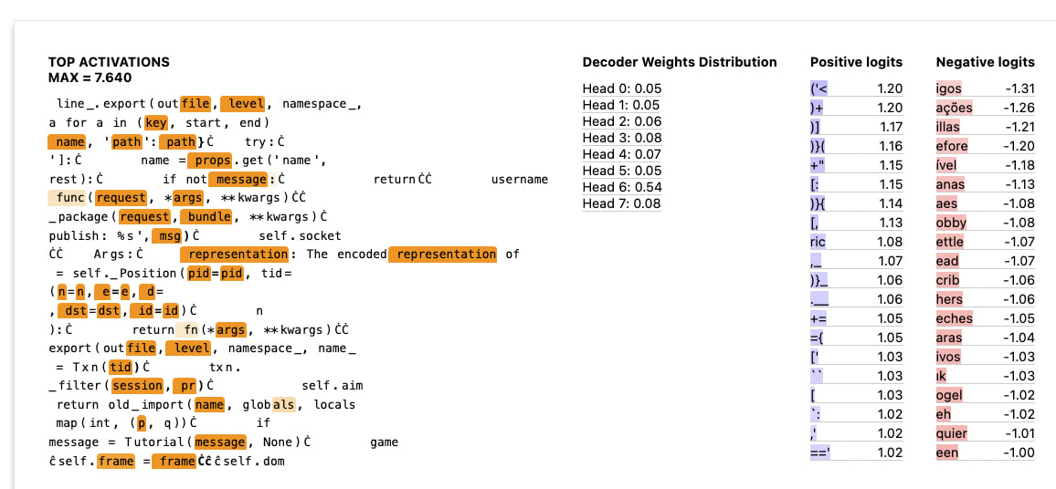

Feature 4635: Prediction of underscores in code, particularly variable names

Feature 12200: Prediction of variable names in code.

Limitations

• Our SAE features had a nontrivial amount of polysemanticity, especially in the lower activation ranges. We suspect we can improve this by using wider SAEs and improving our training (Anthropic-like resampling, more hyperparameter tuning, etc).
• Our proxies were sub-optimal and sometimes had lower correlations than we hoped, causing us to spend lots of time manually starting at false positives / negatives. We think we can improve this by using the GPT 3.5 API to automatically create our proxy masks.

Appendix 

See this Google doc for more details including alternate hypotheses and red teaming.

Citing this work

This is ongoing research. If you want to reference any of our current findings or code, we would appreciate reference to

@misc{attention_saes,
  author= {Connor Kissane and Robert Krzyzanowski and Arthur Conmy and Neel Nanda},
  url = {https://www.alignmentforum.org/posts/DtdzGwFh9dCfsekZZ},
  year = {2024},
  howpublished = {Alignment Forum},
  title = {Sparse Autoencoders Work on Attention Layer Outputs},
}

Author Contributions Statement

Rob and Connor were core contributors on this project and both contributed equally (authorship order chosen arbitrarily). Arthur and Neel gave guidance and feedback throughout the project. The original project idea was suggested by Neel.

1. ^{^}

   Our interface is heavily inspired by Anthropic's and builds on top of Callum McDougall's open source SAE visualizer. We highlight the feature activations in orange, and bold the token directly after the max activating token for each example.  

2. ^{^}

   Note the correlation is between the feature activations and a binary variable (i.e. the boolean proxy masks)

3. ^{^}

   We compute the per-head DFA for each of this features activations on a dataset of 10 million tokens. We calculate of the sum of squares for each head's contributions divided by the total sum of squares (for all contributions)

4. ^{^}

   We also confirm that all of the false positives in the middle activations (2-4) are questions starting with lowercase "which", indicating a flaw in our proxy rather than our high level hypothesis. See appendix for examples.

5. ^{^}

   Note that the DFA analysis suggests head 5 is important, while the decoder weights analysis does not. This a this is a weird anomaly that we don't fully understand.

6. ^{^}

   We decompose the feature contribution from each head into the contribution from each source position, and keep track of the attribution from "Which" source tokens. We then take the ratio of the sum of squares for all the "Which" source token contributions divided by the total sum of squares.

7. ^{^}

   We're not claiming that interpretable outputs are spread across all heads, just that often more than one head per layer is used. See this paper for a high level analysis of how the attention head basis seems somewhat sparse.

8. ^{^}

   Note that there are two additional upstream components that can be used to compute this feature: the positional embeddings and token embeddings. We didn't prioritize these because we expect them to be less interesting, and we were time constrained during the research sprint.

9. ^{^}

   Note that an improved heuristic would incorporate DFA to confirm that most information is sourced from prior B tokens. This was not attempted during the research sprint but will be incorporated in future iterations.