Thanks for the post, I quite enjoyed it! I was especially happy to see the significantly more detailed graphs from the replication than the ones I had seen before.
Re: comparison to my explanation:
I think memorization is actually straightforward for a network to do. You just need a key-value system where the key detects the embedding associated with a given input, then activates the value, which produces the correct output for the detected input. Such systems are easy to implement in many ML architectures (feed forward, convolution, self attention, etc).
I agree this is straightforward for us to understand, but it's still a pretty complicated program that has to be implemented by a large number of parameters, and each individual key-value pair is only reinforced by a single (!!) training data point. Given how little these parameters are being reinforced by SGD, it seems plausible that it only gets to "put 0.95 probability on the answer rather than 0.99".
But more fundamentally, if the memorization circuit was already putting probability ~1 on all the correct answers, then the gradients would be zero and the network would never change (at least in the absence of things like weight decay, and even weight decay often doesn't change circuits when the rest of the gradients are zero). Clearly, the network is changing, therefore the memorized circuit can't be placing probability ~1 on the correct answers.
(This might be wrong if there's some source of gradients other than accuracy / cross-entropy loss. My vague recollection was that grokking happened even when that was the only source of gradients, but I could easily be wrong about that.)
Additionally, it's not the case that "once it hits upon the correctly generalizing function (or something close enough to it), it very quickly becomes confident in it". This is an illusion caused by the log scale on the x-axis of the plots.
Yeah, this was perhaps too much of a simplification. It's more that, at that point in the training process, the gradients are all tiny (since you are mostly predicting the right answer thanks to the memorization). The learning rate might also be significantly lower depending on what learning rate schedule was used; I don't remember the details there. Given that, the speed of learning is striking to me.
Basically, I'm disagreeing with your statement here:
If the model stumbles upon a single general circuit that solves the entire problem, then you'd expect it to make the switch very quickly.
I don't think this is true because thanks to the memorization your gradients are very small and you can't make any switches very quickly.
(It would be interesting to see if, once grokking had clearly started, you could just 100x the learning rate and speed up the convergence to zero validation loss by 100x. That's more strongly predicted by my story; I think it isn't predicted by yours, since you require a more sequential process where circuits get combined over time.)
My account directly predicts that stochasticity and weight decay regularization would help with generalization, and even predicts that weight decay would be one of the most effective interventions to improve generalization.
How so? If you're using the assumption "stochasticity and weight decay probably prefer general circuits over shallow circuits", I feel like given that assumption my story makes the same prediction.
Finally, if we look at a loss plot on a log scale, we can see that the validation loss starts decreasing at ~ step , while the floor on the minimum training loss remains fairly constant (or even increases) until slightly after that (~step ). Thus, validation loss starts decreasing thousands of steps before training loss starts decreasing. Whatever is causing the generalization, it's not doing so to decrease training loss (at least not at first).
Idk what's going on from steps to . I hadn't seen those spikes before, I might interpret them as "failed attempts" to find the one general circuit. I mostly see my story as explaining what happens from onwards. (Notably to me, that's when the validation accuracy looks like it starts increasing.) I do agree this seems like an important piece of data that's not predicted by my story.
I think my biggest reason for preferring my story is actually that it is disanalogous to evolution, and it has complex structures emerging from scratch. Grokking is a really weird phenomenon that you don't usually see in ML systems; I want a weird explanation that wouldn't apply to all the other ML systems that seemingly don't display grokking (e.g. language models).
In addition, it seems like a really big clue that grokking was discovered in this very simple abstract mathematical setting, that seems like exactly the sort of setting where there might be "only two solutions" (memorization and the "true" circuit). I think the "shallow circuits get combined into general circuits" probably is how most neural networks work, and leads to nice smooth loss curves with empirically predictable scaling laws, and is very nicely analogous to evolution -- and this means that usually you don't see grokking; grokking only happens when the structure of the environment means that you can't combine a few shallow circuits into a slightly more general circuit, and instead you have to go directly from "shallow memorization" to "the true answer".
(That being said, an alternative explanation is "the time at which grokking happens increases exponentially with 'complexity' ", which suggests that the simple abstract mathematical setting is the only one in which we'd have trained models far enough to reach the point of grokking.)
I think the general picture here could also explain why RL often has more "jumpy" curves than language models or image classification -- RL is often done in relatively toy environments where there are far fewer features to build circuits out of, relative to language or image data. That being said, "RL has to deal with exploration" is a very plausible alternative explanation for that fact. I do think OpenAI Five and other "big" RL projects had smoother loss curves than more toy RL projects, which supports this picture over "exploration is the problem". Similarly I think this picture can help explain blessings of scale.
It would be interesting to see if, once grokking had clearly started, you could just 100x the learning rate and speed up the convergence to zero validation loss by 100x.
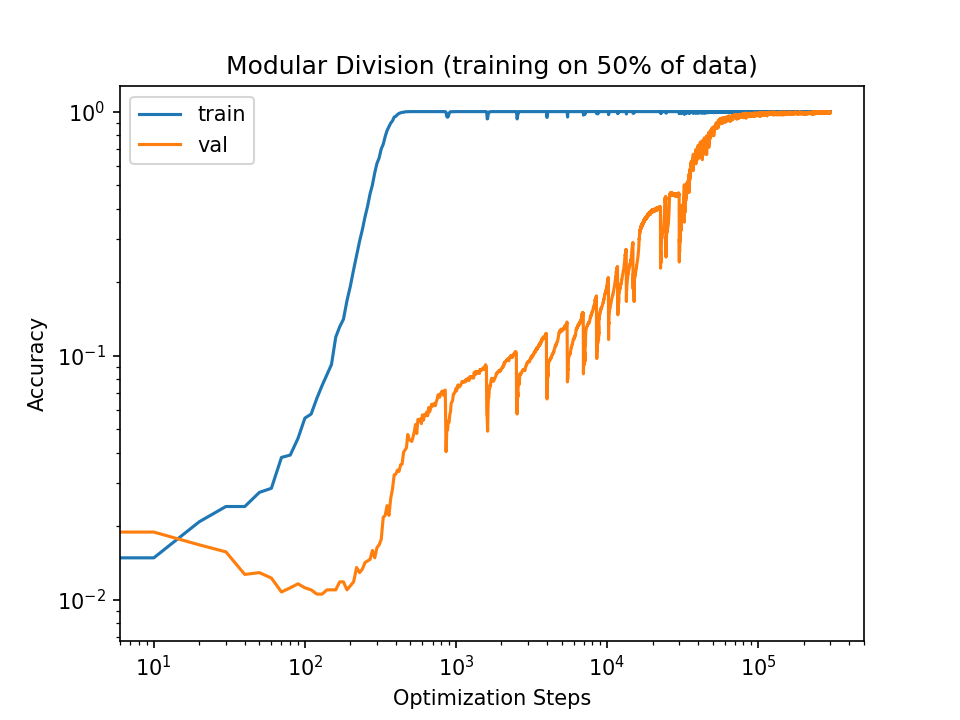
I ran a quick-and-dirty experiment and it does in fact look like you can just crank up the learning rate at the point where some part of grokking happens to speed up convergence significantly. See the wandb report:
I set the LR to 5x the normal value (100x tanked the accuracy, 10x still works though). Of course you would want to anneal it after grokking was finished.
Very nice! Thanks for actually running the experiment :)
It's not clear to me which story this supports since 10x-ing the learning rate only brings the grokking phase down to steps, which is still the majority of the training run.
I'm not sure I understand.
I chose the grokking starting point as 300 steps, based on the yellow plot. I'd say it's reasonable to say that 'grokking is complete' by the 2000 step mark in the default setting, whereas it is complete by the 450 step mark in the 10x setting (assuming appropriate LR decay to avoid overshooting). Also note that the plots in the report are not log-scale
Ah, I just looked at your plots, verified that the grokking indeed still happened with 5x and 10x learning rates, and then just assumed 10x faster convergence in the original plots in the post. Apparently that reasoning was wrong. Presumably you're using different hyperparameters than the ones used in this post? You seem to have faster grokking in the "default setting" than the in the plots shown in the post.
(And it does look like, given some default setting, "10x faster convergence" is basically right, since in your case 10x higher LR makes the grokking stage go from 1700 steps to 150 steps.)
(Partly the issue was that I wasn't sure whether the x-axis in your plots was starting from the beginning of training, or from the point that grokking started, so I instead reasoned about the impact on the graphs in this post. Though looking at the LR plot it's now obvious that it's from the beginning of training.)
I now think this is relatively strong evidence for my view, given that grokking happens pretty quickly (~a third of total training), though it probably is still decently slower than the memorization. (Do you happen to have the training loss curves, so we can estimate how long it takes to memorize under your hyperparameters?)
First, I'd like to note that I don't see why faster convergence after changing the learning rate support either story. After initial memorization, the loss decreases by ~3 OOM. Regardless of what's gaining on inside the network, it wouldn't be surprising if raising the learning rate increased convergence.
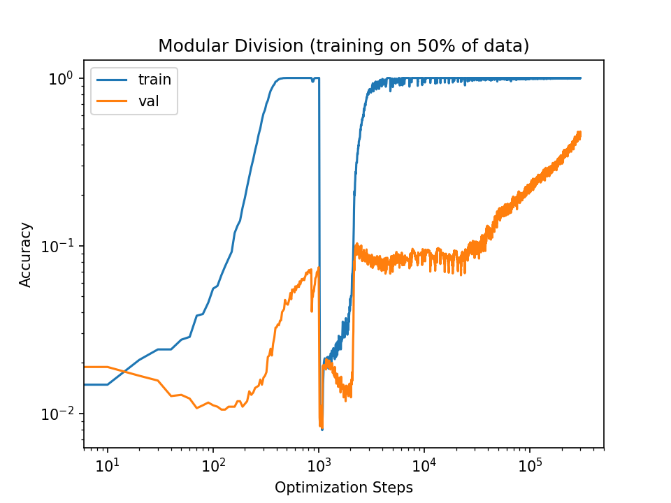
Also, I think what's actually going on here is weirder than either of our interpretations. I ran experiments where I kept the learning rate the same for the first 1000 steps, then increased it by 10x and 50x for the rest of the training.
Here is the accuracy curve with the default learning rate:
Here is the curve with 10x learning rate:
And here is the curve with 50x learning rate:
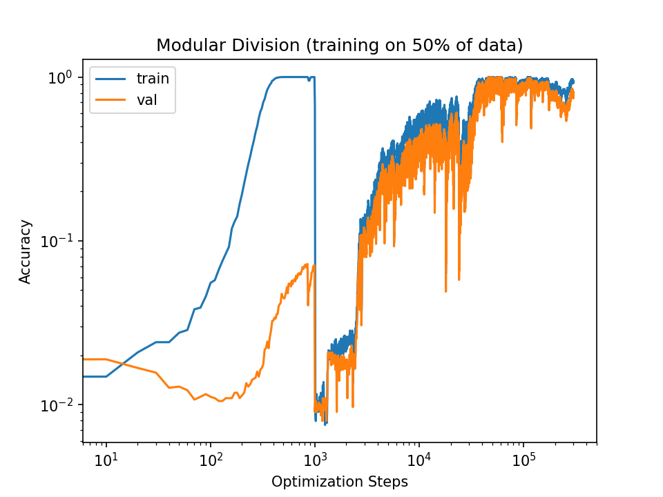
Note that increasing the learning rate doesn't consistently increase validation convergence. The 50x run does reach convergence faster, but the 10x run doesn't even reach it at all.
In fact, increasing the learning rate causes the training accuracy to fall to the validation accuracy, after which they begin to increase together (at least for a while). For the 10x increase, the training accuracy quickly diverges from the validation accuracy. In the 50x run, the training and validation accuracies move in tandem throughout the run.
Frederik's results are broadly similar. If you mouse over the accuracy and loss graphs, you'll see that
- Training performance drops significantly immediately after the learning rate increases.
- The losses and accuracies of the "5x" and "10x" lines correlate together pretty well between training/validation. In contrast, the losses and accuracies of the "default" lines don't correlate strongly between training and testing.
I think that increasing the learning rate after memorization causes some sort of "mode shift" in the training process. It goes from:
First, learn shallow patterns that strongly overfit to the training data, then learn general patterns.
to:
Immediately learn general patterns that perform about equally well on the training and validation data.
In the case of my 10x run, I think it actually has two mode transitions, first from "shallow first" to "immediately general", then another transition back to "shallow first", and that's why you see the training accuracy diverge from the validation accuracy again.
I think results like these make a certain amount of sense, given that higher learning rates are associated with better generalization in more standard settings.
Regardless of what's gaining on inside the network, it wouldn't be surprising if raising the learning rate increased convergence.
I'm kinda confused at your perspective on learning rates. I usually think of learning rates as being set to the maximum possible value such that training is still stable. So it would in fact be surprising if you could just 10x them to speed up convergence. (So an additional aspect of my prediction would be that you can't 10x the learning rate at the beginning of training; if you could then it seems like the hyperparameters were chosen poorly and that should be fixed first.)
Indeed in your experiments at the moment you 10x the learning rate accuracy does in fact plummet! I'm a bit surprised it manages to recover, but you can see that the recovery is not nearly as stable as the original training before increasing the learning rate (this is even more obvious in the 50x case), and notably even the recovery for the training accuracy looks like it takes longer (1000-2000 steps) than the original increase in training accuracy (~400 steps).
I do think this suggests that you can't in fact "just 10x the learning rate" once grokking starts, which seems like a hit to my story.
I updated the report with the training curves. Under default settings, 100% training accuracy is reached after 500 steps.
There is actually an overlap between the train/val curves going up. Might be an artifact of the simplicity of the task or that I didn't properly split the dataset (e.g. x+y being in train and y+x being in val). I might run it again for a harder task to verify.
Huh, intriguing. Yeah, it might be worth running with a non-commutative function and seeing if it holds up -- it seems like in the default setting the validation accuracy hits almost 0.5 once the training accuracy is 1, which is about what you'd get if you understood commutativity but nothing else about the function. So the "grokking" part is probably happening after that, i.e. at roughly the 1.5k steps location in the default setting.
So I ran some experiments for the permutation group S_5 with the task x o y = ?
Interestingly here increasing the learning rate just never works. I'm very confused.
Also interestingly, in the default setting for these new experiments, grokking happens in ~1000 steps while memorization happens in ~1500 steps, so the grokking is already faster than the memorization, in stark contrast to the graphs in the original post.
(This does depend on when you start the counter for grokking, as there's a long period of slowly increasing validation accuracy. You could reasonably say grokking took ~2500 steps.)
Oh I thought figure 1 was S5 but it actually is modular division. I'll give that a go..
Here are results for modular division. Not super sure what to make of them. Small increases in learning rate work, but so does just choosing a larger learning rate from the beginning. In fact, increasing lr to 5x from the beginning works super well but switching to 5x once grokking arguably starts just destroys any progress. 10x lr from the start does not work (nor when switching later)
So maybe the initial observation is more a general/global property of the loss landscape for the task and not of the particular region during grokking?
Yeah, that seems right, I think I'm basically at "no, you can't just 10x the learning rate once grokking starts".
Yep I used my own re-implementation, which somehow has slightly different behavior.
I'll also note that the task in the report is modular addition while figure 1 from the paper (the one with the red and green lines for train/val) is the significantly harder permutation group task.
Summary: I discuss a potential mechanistic explanation for why SGD might prefer general circuits for generating model outputs. I use this preference to explain how models can learn to generalize even after overfitting to near zero training error (i.e., grokking). I also discuss other perspectives on grokking and deep learning generalization.
Additionally, I discuss potential experiments to confirm or reject my hypothesis. I suggest that a tendency to unify many shallow patterns into fewer general patterns is a core feature of effective learning systems, potentially including humans and future AI, and briefly address implications to AI alignment.
Epistemic status: I think the hypothesis I present makes a lot of sense and is probably true, but I haven't confirmed things experimentally. Much of my motive for post this is to clarify my own thinking and get feedback on the best ways to experimentally validate this perspective on ML generalization.
Context about circuits: This post assumes the reader is familiar with and accepts the circuits perspective on deep learning. See here for a discussion of circuits for CNN vision models and here for a discussion of circuits for transformer NLP models.
Evidence from grokking
The paper "Grokking: Generalization Beyond Overfitting on Small Algorithmic Datasets" uses stochastic gradient descent (SGD) to train self attention based deep learning models on different modular arithmetic expressions (e.g., f(x,y)=x×y (mod p), where p is fixed).
The training data only contain subsets of the function's possible input/output pairs. Initially, the models overfit to their training data and are unable to generalize to the validation input/output pairs. In fact, the models quickly reach near perfect accuracy on their training data. However, training the model for significantly past the point of overfitting causes the model to generalize to the validation data, what the authors call "grokking".
See figure 1a from the paper:
Note the model has near perfect accuracy on the training data. Thanks to a recent replication of this work, we can also look at the loss curves during grokking (though on a different experiment compared to the plot above):
First, the model reaches near-zero loss in training but overfits in validation. However, the validation loss soon starts decreasing until the model correctly classifies both the validation and training data.
This brings up an interesting question: why did the model learn anything at all after reaching near zero loss on the training data? Why not just stick with memorizing the training data? What would prompt SGD to switch over to general circuitry that solves both training and validation data?
I think the answer is surprisingly straightforward: SGD prefers general circuits because general circuits make predictions on a greater fraction of the training data. Thus, general circuits receive more frequent SGD reinforcement for making correct predictions. Think of each data point as "pushing" the model to form circuits that perform well on that data point. General circuits perform well on many data points, so they receive a greater "push" towards forming.
Shallow circuits are easier to form with SGD, but they aren't retained as strongly. Thus, as training progresses, general circuits eventually overtake the shallow circuits.
Toy example of SGD preferring general circuits
Let's consider a toy example of memorizing two input/output pairs. Suppose:
One way the model might memorize the these data points is to use two independent, shallow circuits, one for each data point. I show a diagram of how this might be implemented using two different self attention heads:
(Suppose for simplicity that these attention heads ONLY implement the circuit shown)
W1QK and W2QK represent the query-key[1] circuits associated with their associated attention heads. W1QK and W2QK are respectively searching for x1,y1 and x2,y2 appearing in the input, and trigger their respective output-value[1] circuits - represented by W1OV and W2OV - when they find their desired inputs.
Another way to memorize these data points is to use a more general, combined circuit implemented with a single attention head:
Here, W1+2QK represents a single query-key circuit that looks for either x1,y1 or x2,y2 in the input and triggers the output-value circuit W1+2OV to produce either output 1 or output 2 depending on the triggering input.
I think SGD will prefer the single general circuit to the shallow circuits because the general circuit produces correct predictions on a greater fraction of the input examples. SGD only reinforces one of the shallow circuits when the model processes the specific input associated with that circuit. In contrast, SGD reinforces the general circuit whenever the model processes either of the inputs for which the general circuit produces correct predictions.
To clarify: both circuit configurations described here memorize the data, and both would likely fail completely on validation data. The single circuit that memorizes both datapoints is more “general” in the sense that it generates more total correct predictions. I use memorizing circuits as my examples here to highlight the fact that I use “generality” to refer specifically to the number of training datapoints for which a circuit generates correct predictions, not, say, the probability that a circuit generalizes from the training data to the validation data.
Another way to see why SGD would prefer the general circuit: catastrophic forgetting is the tendency of models initially trained on task A, then trained on task B to forget task A while learning task B. Consider that, if the model isn't processing inputs containing x1,y1, the individaul circuit that produces output 1 will experience catestrophic forgetting. Thus, all training examples except one are degrading the shallow circuit's performance.
In contrast, the general circuit generates predictions for both x1,y1 and x2,y2. It's reinforced twice as frequently, so it's better able to recover from degradation caused by training on the other examples. Eventually, the general circuit subsumes the functionality of the two shallow circuits.
From figure 2a of "Grokking: Generalization Beyond Overfitting on Small Algorithmic Datasets", we can see that stochasticity and regularization significantly speeds up generalization. Potentially, this occurs because both randomness in the SGD updates and weight decay help to degrade shallow circuits, allowing general circuits to more quickly dominate. I think a large amount of weight decay's value in other domains comes from it degrading shallow circuits more than general circuits.
I think the conceptual arguments I've provided above strongly imply that SGD has some sort of preference for general circuits over a functionally equivalent collection of shallow circuits. In this next section, I try to flush out in more detail how this might manifest in the training process. However, I think this section is more speculative than the arguments above.
Significance for the entire model
The process of unifying multiple shallow circuits into fewer, more general circuits happens at multiple levels throughout the training process. Gradually, the shallow circuits combine into slightly more general circuits, which themselves combine further. Eventually, all the shallow memorization circuits combine into a single circuit representing the true modular arithmetic expression.
I think we see artifacts of this combination process in the grokking loss plots, specifically in the spikes:
Note that each loss spike in the training data corresponds with a loss spike in the validation data. I think these spikes represent unification events where the model replaces multiple shallow circuits with a smaller number of more general circuits.
The previous section described general vs shallow circuits as a binary choice, with the model able to use either one general circuit or a collection of shallow circuits. However, real deep learning models are more complex. They can simultaneously implement multiple instances of both types of circuits, with each circuit being partially responsible for a part of a single prediction.
Let's consider Dn={d1,...,dn} and representing a subset of the training data.
For the start of the training, I think each prediction on the elements of Dn is mainly generated by multiple different shallow circuits, with some small fraction of each prediction coming from a single partially implemented general circuit.
As training progresses, the model gradually refines whatever general circuit contributes to correct predictions on all of Dn. Eventually, the model reaches an inflection point where it has a general circuit that can correctly predict all of Dn. At this point, I think there's a relatively quick phase shift in which the general circuit substitutes in for multiple shallow circuits at once. These shifts generate the loss spikes seen in the plot above.
I'm unsure why switching from shallow to general circuits would cause a loss spike. I suspect the network is encountering something like a renormalization issue. The general circuit may be generating predictions for Dn, but that doesn't mean that all of the shallow circuits have been removed. If there are elements of Dn where both the general circuit and its original shallow circuit generate predictions, that may cause the network to behave poorly on those data points.
Generalization to validation data starts to happen when the only way for the model to fit more correct predictions into a single circuit is for that circuit to actually start modeling the underlying data generating process. This leads to circuits that are still shallow, but have some limited generalization capability.
To see how a model might implement partially generalizing shallow patterns, imagine a circuit using a linear approximation to f(x,y)=x×y (mod p) as g(x,y)=x×y to efficiently store many predictions on the training data. Note this approximation is correct so long as x×y<p, so it does have some degree of generalization to validation data, even though the model only learned it for training data. Similarly, the network can use g(x,y)=x×y−m×p for any (x,y) such that x×y∈[m×p,m(p+1)).
Midway through grokking, the network probably looks an ensemble of circuits that each represent the true data distribution in different areas of the input space. Eventually, these partially generalizing shallow patterns combine together into a single circuit that correctly represents the true arithmetic expression (e.g., by first computing m as a function of x×y, then feeding that m into g(x,y,m)=x×y−m×p.
Other explanations of grokking
Grokking: Generalization Beyond Overfitting on Small Algorithmic Datasets doesn't offer any particular interpretation of their results. However, Rohin's summary of the paper proposed the following:
I strongly prefer my account of grokking for several reasons.
(I also think it's interesting how regular the training loss spikes look from steps 2×10³ to 104. There's a sharp jump, followed by a sharp decrease, then a shallower decrease, then another spike almost immediately after. I have no idea what to make of it, but whatever underlying mechanism drives this behavior should be interesting.)
Rohin's explanations is the only other attempted explanation of grokking I've seen. Please let me know of any more in the comments.
Other explanations of generalization
Prior work has proposed that neural network generalization happens primarily as a result of neural network initializations strongly favoring simpler functions, with relatively little inductive bias coming from the optimization procedure.
E.g., Is SGD a Bayesian sampler? Well, almost demonstrated that if you randomly sample neural network initializations until you find one that has low error on a training set, that network will generalize to the test data. Additionally, the test set predictions made by the randomly sampled classifier will correlate strongly with the test set predictions make by a classifier learned via SGD.
I think such work clearly demonstrates that network initializations are strongly biased towards simple functions. However, I think these results are compatible with SGD having a bias towards general circuits.
For one, common patterns in data may explain common patterns in models fit to that data. The correlation between SGD learned and randomly sampled classifiers seem to be a specific instance of the tendency for many types of learning to converge to exhibit similar behavior when trained on similar data. I.e., both SGD and randomly sampled classifiers seem less likely to fit outlier datapoints and more likely to fit tightly clustered datapoints.
Additionally, generality bias seems similar to simplicity bias. Occam's razor implies simpler circuits are more likely to generalize. All else equal, general circuit are more likely to be simple. Potentially, the only difference between the "simplicity bias from initialization" vs "simplicity bias from initialization and generality bias from SGD" perspectives on generalization is that the latter implies faster learning than the former. Perhaps not-coincidentally, SGD is one of the fastest ways to train neural nets.
Experimental investigations
Given a particular output from a neural net, there are methods of determining which neurons are most responsible for generating that output. Such scores are often called the "saliency" of a given neuron for a particular output. Example methods include integrated gradients and Shapley values.
I think we can find experimental evidence for or against the general circuits hypothesis by looking at how the distribution over neuron saliencies evolves during training. When shallow circuits dominate network behavior, each neuron will mostly be salient for generating a small fraction of the outputs. However, as more general circuits form, there should be a small collection of neurons that become highly salient for many different outputs. We should be able to do something like look at a histogram of average neuron saliencies measured across many inputs.
One idea is to record neuron saliencies for each prediction in each training/testing epoch, then compute the median saliency for each neuron in each epoch. After which, I'll generate a histogram of the neurons' median saliencies for each epoch. I should see the histogram becoming more and more right-skewed as the training progresses. This should happen because general circuits are salient for a greater fraction of the inputs.
Another idea would be to find the k neurons with the highest saliency at each epoch, then test what happens if we delete them. As training progresses, individual circuits will become responsible for a greater fraction of the model's predictions. We should find that this deletion operation damages more and more of the model's predictive capability.
Both these ideas would provide evidence for general circuits replacing shallow circuits over time. However, they'd not show that the specific reason for this replacement was because general circuits made more predictions and so were favored by SGD. I'm unsure how to investigate this specific hypothesis. All I can think of is to identify some set of shallow circuits and a single general circuit that makes the same predictions as the set of shallow circuits. Then, record the predictions and gradients made by the shallow and general circuits and hope to find a clear, interpretable pattern of the general circuit receiving more frequent/stronger updates and gradually replacing the shallow circuits.
(If anyone can think about other experimental investigations or has thoughts on this proposal, please share in the comments!)
Implications for learning in general
My guess is that many effective learning systems will have heuristics that cause them to favor circuits that make lots of predictions.
For example, many tendencies of the brain seem to promote general circuitry. Both memories and skills decay over time unless they're periodically refreshed. When senses are lost, the brain regions corresponding to those senses are repurposed towards processing the remaining sense data.
In addition to using low-level processes that promote general circuitry, highly capable learning systems may develop a high-level tendency towards generalization because such a tendency is adaptive for many problems. In other words, they may learn to "mesa-generalize"[2].
I think humans show evidence of a mesa-generalization instinct. Consider that religions, ideologies, philosophical frameworks and conspiracy theories often try to explain a large fraction of the world through a single lens. Many such grand narratives make frequent predictions about hard to verify things. Without being able to easily verify those predictions, our mesa generalization instincts may favor narratives that make many predictions.
Potentially, ML systems will have a similar mesa-generalization instinct. This could be a good thing. Human philosophers have put quite a bit of effort into mesa-generalizing a universal theory of ethics. If ML systems are naturally inclined to do something similar, maybe we can try to point this process in the right direction?
Mesa-generalization from ML systems could also be dangerous, for much the same reason mesa-optimization is dangerous. We don't know what sort of generalization instinct the system might adopt, and it could influence the system's behaviors in ways that are hard to predict from the training data.
This seems related to the natural abstractions hypothesis. Mesa-generalization suggests an ML system should prefer frequently used abstractions. At a human level of capabilities, these should coincide reasonably well with human abstractions. However, more capable systems are presumably able to form superhuman abstractions that are used for a greater fraction of situations. This suggests we might have initially encouraging "alignment by default"-type results, only for the foundation of that approach to collapse as we reach superhuman capabilities.
Essentially, the query-key circuit determines which input tokens are most important, and the output-value circuit determines which outputs to generate for each attended token. See "A Mathematical Framework for Transformer Circuits" for more details on query-key / output-value formulation of self attention.
So named after "mesa-optimization", the potential for learning systems to implement an optimization procedure as an adaptive element of their cognition. See Risks from Learned Optimization in Advanced Machine Learning Systems.