Author's Note: This post is a bunch of mathy research stuff with very little explanation of context. Other posts in this sequence will provide more context, but you might want to skip this one unless you're looking for mathy details.
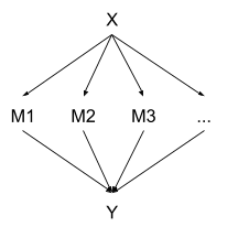
Suppose we have a medical sensor measuring some physiological parameter. The parameter has a constant true value , and the sensor takes measurements over a short period of time. Each measurement has IID error (so the measurements are conditionally independent given ). In the end, the measurements are averaged together, and there’s a little bit of extra error as the device is started/stopped, resulting in the final estimate - the only part displayed to the end user. We can represent all this with a causal DAG:

Note that, conceptually, there are two main sources of error in the final estimate Y:
- IID measurement noise in the ’s
- Noise in Y from the starting/stopping procedure
… so the node is not fully deterministic. The joint distribution for the whole system is given by
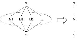
Since all the measurements are to be averaged together anyway, it would be nice if we could just glom them all together and treat them as a single abstract measurement, like this:

Formally, we can do this in two steps:
- Replace the nodes with a single node , i.e. a list containing all the measurements. This doesn’t change the substance of the model at all, it just changes what we’re calling a “node”.
- Replace the node with , the average of the measurements. We no longer worry about the individual measurements at all, and just directly compute the distributions and .
The second step is the interesting one, since it changes the substance of the model.
Main question: under the abstract model, what counterfactual queries remain valid (i.e. match the corresponding concrete queries), and how do they correspond to counterfactuals on the concrete model? What about probabilistic queries, like ?
The concrete model supports three basic counterfactual queries:
- Set the value of
- Set the value of
- Set the value of
… as well as counterfactuals built by combining multiple basic counterfactuals and possibly adding additional computation. In the abstract model:
- Setting abstract works exactly the same and corresponds directly to the concrete-model counterfactual.
- Although the abstract node has different inputs and computation than the concrete node, the procedure for setting abstract is exactly the same: cut all the incoming arrows and set the value.
- Setting corresponds to setting all of the concrete at once, and there may be degeneracy: a single counterfactual setting of may correspond to many possible counterfactual settings of the whole set of measurements .
… so counterfactuals on and have a straightforward correspondence, whereas the correspondence between counterfactuals on and is more complicated and potentially underdetermined. But the important point is that any allowable counterfactual setting of will correspond to at least one possible counterfactual setting of - so any counterfactual queries on the abstract model are workable.
(Definitional note: I’m using “correspond” somewhat informally; I generally mean that there’s a mapping from abstract nodes to concrete node sets such that queries on the abstract model produce the same answers as queries on the concrete model by replacing each node according to the map.)
Probabilistic queries, i.e. , run into a more severe issue: . In the abstract model, node retained all information relevant to , but not necessarily all information relevant to . So there’s not a clean correspondence between probabilistic queries in the two models. Also, of course, the abstract model has no notion at all of the individual measurements , so it certainly can’t handle queries like .
Now, in our medical device example, the individual measurements are not directly observed by the end user - they just see - so none of this is really a problem. The query will never need to be run anyway. That said, a small adjustment to the abstract model does allow us to handle that query.
Natural Abstraction for the Medical Sensor
Let’s modify our abstract model from the previous section so that . Rather than just keeping the information relevant to , our node will also need to keep information relevant to . (The next three paragraphs briefly explain how to do this, but can be skipped if you're not interested in the details.)
By the minimal map theorems, all the information in which is relevant to is contained in the distribution . So we could just declare that node is the tuple , where the second item is the full distribution of given (expressed as a function). But notation gets confusing when we carry around distributions as random variables in their own right, so instead we’ll simplify things a bit by assuming the measurements follow a maximum entropy distribution - just remember that this simplification is a convenience, not a necessity.
We still need to keep all the information in which is relevant to , which means we need to keep all the information to compute . From the DAG structure, we know that , where is a normalizer. is part of the model, so the only information we need from to compute is the product . If we assume the measurements follow a maxentropic distribution (for simplicity), then , for some vector and vector-valued function (both specified by the model). Thus, all we need to keep around to compute is - the sufficient statistic.
Main point: the node consists of the pair . If we want to simplify even further, we can just declare that is the identity function (possibly with ), and then node is just , assuming the number of measurements is fixed.
What does this buy us?
First and foremost, our abstract model now supports all probabilistic queries: , , , , etc, will all return the same values as the corresponding queries on the concrete model (with corresponding to ). The same counterfactuals remain valid with the same correspondences as before, and the counterfactually-modified abstract models will also support the additional probabilistic queries.
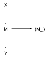
We can even add in one extra feature:

Huh? What’s going on here?
Remember, contains all of the information from which is relevant to or . That means is conditionally independent of both and , given (this is a standard result in information theory). So we can add into the DAG as a child of M, resulting in the overall distribution
Since is just a child node dangling off the side, any probabilistic queries not involving any will just automatically ignore it. Any probabilistic queries which do involve any will incorporate relevant information from and via .
What about counterfactuals?
Counterfactual settings of , , and still work just like before, and we can generally run probabilistic queries involving the on the counterfactually-modified DAGs. Cutting the arrow still corresponds to cutting all the arrows in the concrete model. The addition of to the model even lets us calculate which are compatible with a particular counterfactual setting of , although I don’t (yet) know of any useful interpretation to attribute to the distribution in that case.
We still can’t directly translate counterfactuals from the concrete model to the abstract model - e.g. a counterfactual setting of in the concrete model does not easily correspond to anything in the abstract model. We also can’t directly run counterfactuals on in the abstract model; we have to run them on instead. But if a counterfactual modification is made elsewhere in the DAG, the probabilistic queries of within the counterfactual model will work.
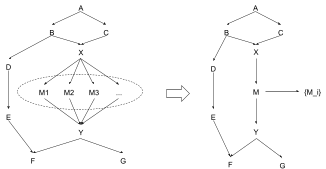
That brings us to the most important property of this abstraction, and the real reason I call it “natural”: what if this is all just a sub-component of a larger model?

Here’s the beauty of it: everything still works. All probabilistic queries are still supported, all of the new counterfactuals are supported. And all we had to account for was the local effects of our abstraction - i.e. had to contain all the information relevant to and . (In general, an abstracted node needs to keep information relevant to its Markov blanket.) Any information relevant to anything else in the DAG is mediated by and/or , so all of our transformations from earlier still maintain invariance of the relevant queries, and we’re good.
By contrast, our original abstraction - in which we kept the information relevant to but didn’t worry about - would mess up any queries involving the information contained in relevant to . That includes , , etc. To compute those correctly, we would have had to fall back on the concrete model, and wouldn’t be able to leverage the abstract model at all. But in the natural abstraction, where contains all information relevant to or , we can just compute all those queries directly in the abstract model - while still gaining the efficiency benefits of abstraction when possible.