Say we have two events, $A$ and $B$, and a probability distribution $P$ over whether or not they happen. We can represent $P$ as a square:

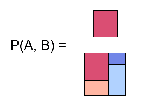
So for example, the probability $P(A,B)$ of both $A$ and $B$ occurring is the ratio of [the area of the dark red region] to [the area of the entire square]:

Visualizing probabilities in a square is neat because we can draw simple pictures that highlight interesting facts about our probability distribution.

Below are some pictures illustrating:

• independent events (What happens if the columns and the rows in our square both line up?)

• marginal probabilities (If we're looking at a square of probabilities, where's the probability $P\left(A\right)$ of $A$ or the probability $P\left(\neg B\right)$?)

• conditional probabilities (Can we find in the square the probability $P(B\mid A)$ of $B$ if we condition on seeing $A$? What about the conditional probability $P(A\mid B)$?)

• factoring a distribution (Can we always write $P$ as a square? Why do the columns line up but not the rows?)

• the process of computing joint probabilities from factored probabilities

Independent events

Here's a picture of the joint distribution of two independent events $A$ and $B$:

Now the rows for $P\left(B\right)$ and $P\left(\neg B\right)$ line up across the two columns. This is because $P(B\mid A)=P\left(B\right)=P(B\mid \neg A)$. When $A$ and $B$ are independent, updating on $A$ or $\neg A$ doesn't change the probability of $B$.

For more on this visualization of independent events, see the aptly named Two independent events: Square visualization.

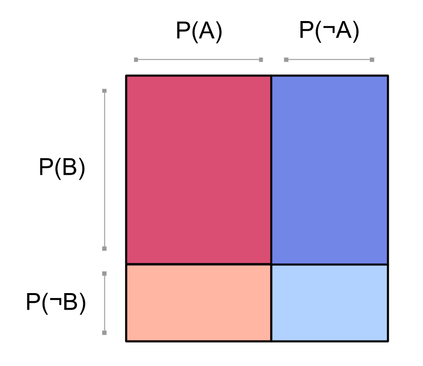
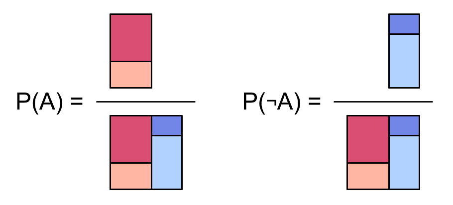
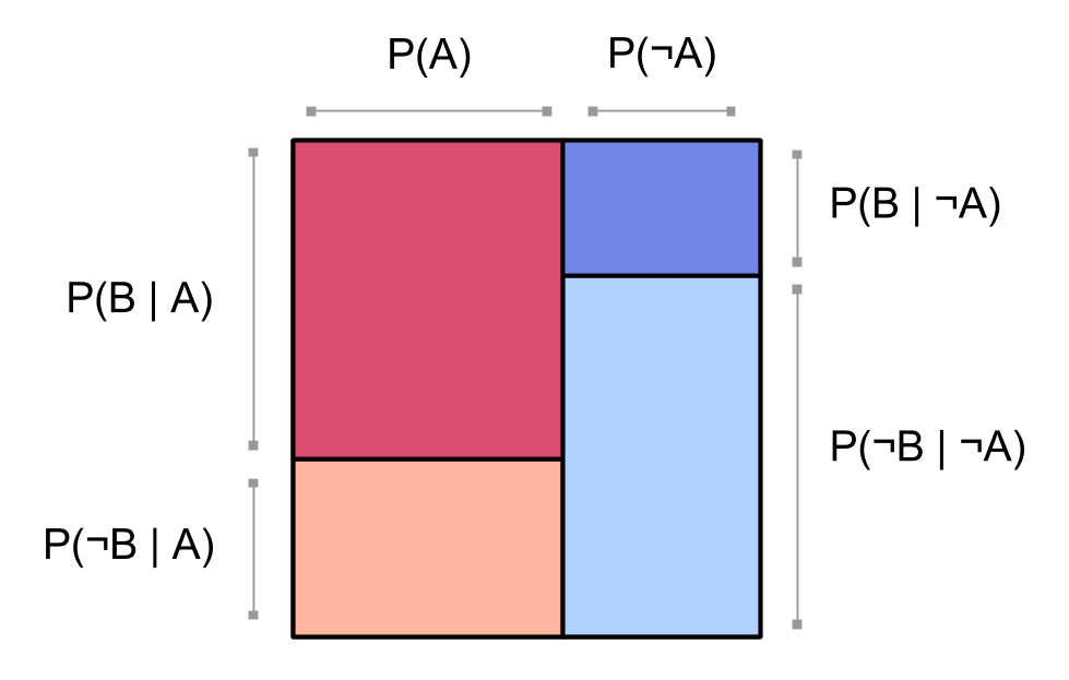
Marginal probabilities

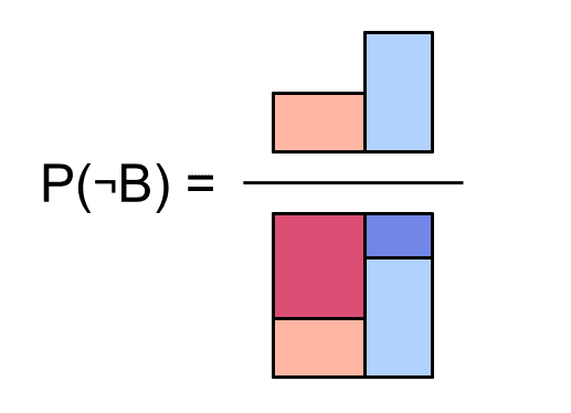
We can see the marginal probabilities of $A$ and $B$ by looking at some of the blocks in our square. For example, to find the probability $P\left(\neg A\right)$ that $A$ doesn't occur, we just need to add up all the blocks where $\neg A$ happens: $P\left(\neg A\right)=P(\neg A,B)+P(\neg A,\neg B)$.

Here's the probability $P\left(A\right)$ of $A$, and the probability $P\left(\neg A\right)$ of $\neg A$:

Here's the probability $P\left(\neg B\right)$ of $\neg B$:

In these pictures we're dividing by the area of the whole square. Since the probability of anything at all happening is 1, we could just leave it out, but it'll be helpful for comparison while we think about conditionals next.

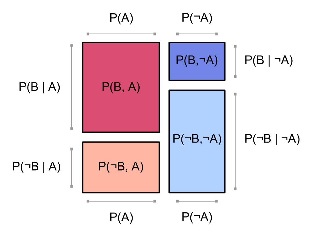
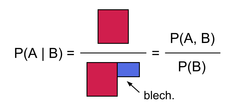
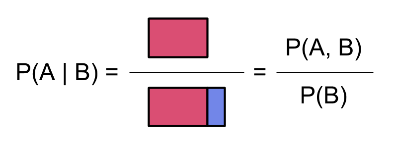
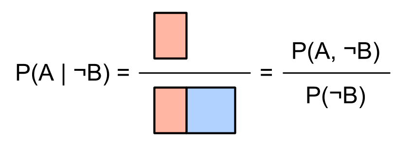
Conditional probabilities

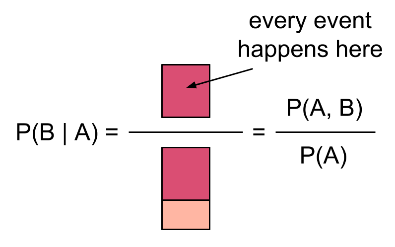
We can start with some probability $P\left(B\right)$, and then assume that $A$ is true to get a conditional probability $P(B\mid A)$ of $B$. Conditioning on $A$ being true is like restricting our whole attention to just the possible worlds where $A$ happens:

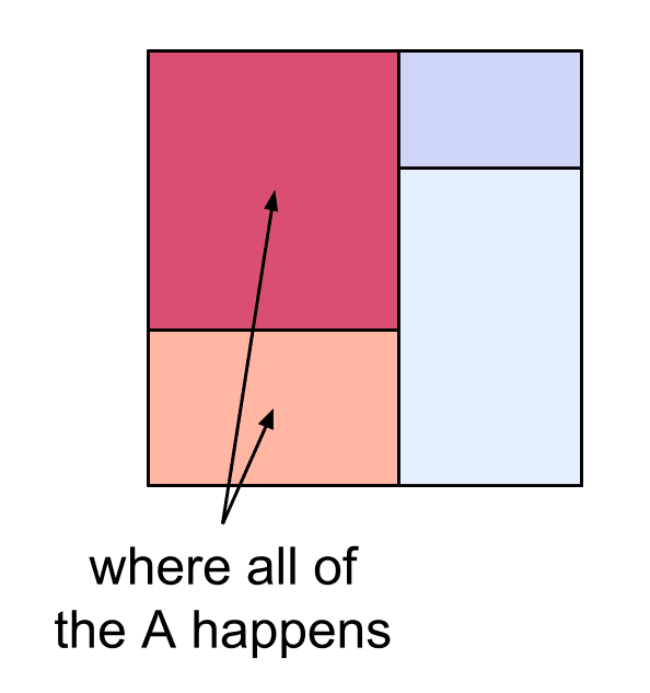
Then the conditional probability of $B$ given $A$ is the proportion of these $A$ worlds where $B$ also happens:

If instead we condition on $\neg A$, we get:

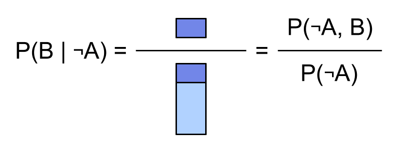
So our square visualization gives a nice way to see, at a glance, the conditional probabilities of $B$ given $A$ or given $\neg A$:

We don't get such nice pictures for $P(A\mid B)$:

More on this next.

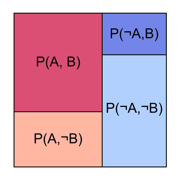
Factoring a distribution

Recall the square showing our joint distribution $P$:

Notice that in the above square, the reddish blocks for $P(A,B)$ and $P(A,\neg B)$ are the same width and form a column; and likewise the blueish blocks for $P(\neg A,B)$ and $P(\neg A,\neg B)$. This is because we chose to factor our probability distribution starting with $A$:

$$P(A,B)=P\left(A\right)P(B\mid A).$$

Let's use the equivalence between events and binary random variables, so if we say $P(B=\text{True}\mid A=\text{False})$ we mean $P(B\mid \neg A)$. For any choice of truth values $t_A\in \{\text{True},\text{False}\}$ and $t_B\in \{\text{True},\text{False}\}$, we have

$$P(A=t_A,B=t_B)=P(A=t_A)P(B=t_B\mid A=t_A).$$

The first factor $P(A=t_A)$ tells us how wide to make the red column $\left(P\right(A=\text{True}\left)\right)$ relative to the blue column $\left(P\right(A=\text{False}\left)\right)$. Then the second factor $P(B=t_B\mid A=t_A)$ tells us the proportions of dark $(B=\text{True})$ and light $(B=\text{False})$ within the column for $A=t_A$.

We could just as well have factored by $B$ first:

$$P(A=t_A,B=t_B)=P(B=t_B)P(A=t_A\mid B=t_b).$$

Then we'd draw a picture like this:

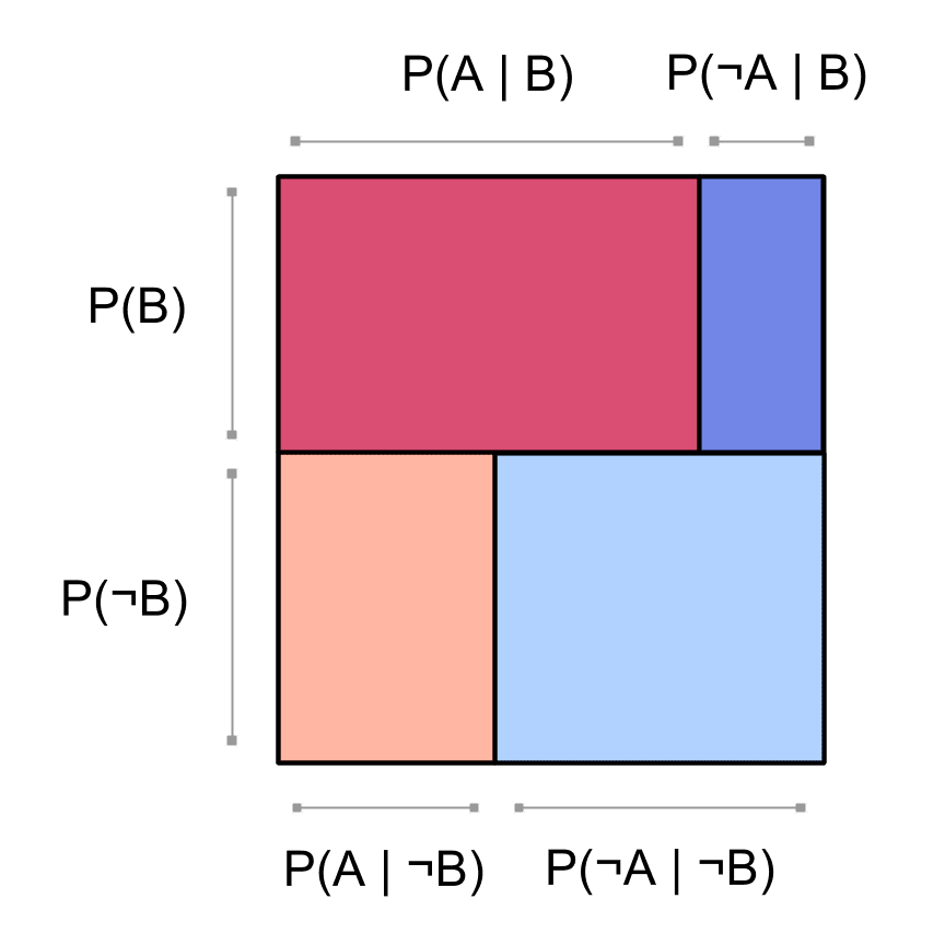
By the way, earlier when we factored by $A$ first, we got simple pictures of the probabilities $P(B\mid A)$ for $B$ conditioned on $A$. Now that we're factoring by $B$ first, we have simple pictures for the conditional probability $P(A\mid B)$:

and for the conditional probability $P(A\mid \neg B)$:

Computing joint probabilities from factored probabilities

Let's say we know the factored probabilities for $A$ and $B$, factoring by $A$. That is, we know $P(A=\text{True})$, and we also know $P(B=\text{True}\mid A=\text{True})$ and $P(B=\text{True}\mid A=\text{False})$. How can we recover the joint probability $P(A=t_A,B=t_B)$ that $A=t_A$ is the case and also $B=t_B$ is the case?

Since

$$P(B=\text{False}\mid A=\text{True})=\frac{P(A=\text{True},B=\text{False})}{P(A=\text{True})},$$

we can multiply the prior $P\left(A\right)$ by the conditional $P(\neg B\mid A)$ to get the joint $P(A,\neg B)$:

$$P(A=\text{True})P(B=\text{False}\mid A=\text{True})=P(A=\text{True},B=\text{False}).$$

If we do this at the same time for all the possible truth values $t_A$ and $t_B$, we get back the full joint distribution: