Lewis Smith*, Sen Rajamanoharan*, Arthur Conmy, Callum McDougall, Janos Kramar, Tom Lieberum, Rohin Shah, Neel Nanda

* = equal contribution

The following piece is a list of snippets about research from the GDM mechanistic interpretability team, which we didn’t consider a good fit for turning into a paper, but which we thought the community might benefit from seeing in this less formal form. These are largely things that we found in the process of a project investigating whether sparse autoencoders (SAEs) were useful for downstream tasks, notably out-of-distribution probing.

TL;DR

• To validate whether SAEs were a worthwhile technique, we explored whether they were useful on the downstream task of OOD generalisation when detecting harmful intent in user prompts
• Negative result: SAEs underperformed linear probes
  • Corollary: Linear probes are actually really good and cheap and perform great
• As a result of this and parallel work, we are deprioritising fundamental SAE research for the moment and exploring other directions, though SAEs will remain a tool in our toolkit
  • We do not think that SAEs are useless or that no one should work on them, but we also do not think that SAEs will be a game-changer for interpretability, and speculate that the field is over-invested in them.
• Training SAEs specialised for chat data closed about half the gap but was still worse than linear probes
  • We tried several ways to train chat SAEs, all did about as well. By default, we recommend taking an SAE on pretraining data and finetuning it on a bit of chat data
• Other results:
  • We found SAEs fairly helpful for debugging low quality datasets (noticing spurious correlations)
  • We present a variant of JumpReLU with an alternative sparsity penalty to get rid of high-frequency latents
  • We argue that a standard auto-interp approach of computing the average interpretability of a uniformly sampled SAE latent can be misleading as it doesn’t penalise models which have high frequency, but not very interpretable, latents, and explore weighting the interpretability score by latent frequency.

Introduction

Motivation

Our core motivation was that we, along with much of the interpretability community, had invested a lot of our energy into Sparse Autoencoder (SAE) research. But SAEs lack a ground truth of the “true” features in language models to compare to, making it pretty unclear how well they work. There is qualitative evidence that SAEs are clearly doing something, far more structure than you would expect by random chance. But they clearly have a bunch of issues: if you just type an arbitrary sentence into Neuronpedia, and look at the latents that light up, they do not seem to perfectly correspond to a crisp explanation.

More generally, when thinking about whether we should prioritise working on SAEs, it's worth thinking about how to decide what kind of interpretability research to do in general. One perspective is to assume there is some crisp, underlying, human-comprehensible truth for what is going on in the model, and to try to build techniques to reverse engineer it. In the case of SAEs, this looks like the hope that SAE latents capture some canonical set of true concepts inside the model. We think it is clear now that SAEs in their current form are far from achieving this, and it is unclear to us if such “true concepts” even exist. There are several flaws with SAEs that prevent them from capturing a true set of concepts even if one exists, and we are pessimistic that these can all be resolved:

• SAEs are missing concepts
• Concepts are represented in noisy ways where e.g. small activations don't seem interpretable
• Latents can be warped in weird ways like feature absorption
• Seemingly interpretable latents have many false negatives.
• For more issues with SAEs see Section 2.1.2c of Sharkey et al.

But there are other high-level goals for interpretability than perfectly finding the objective truth of what’s going on - if we can build tools that give understanding that’s imperfect but enough to let us do useful things, like understand whether a model is faking alignment, that is still very worthwhile. Several important goals, like trying to debug mysterious failures and phenomena, achieving a better understanding of what goals and deception look like, or trying to detect deceptive alignment, do not necessarily require us to discover all of the ‘true features’ of a model; a decent approximation to the models computation might well be good enough. But how could we tell if working on SAEs was bringing us closer to these goals?

Our hypothesis was that if SAEs will eventually be useful for these ambitious tasks, they should enable us to do something new today. So, the goal of this project was to investigate whether we can do anything useful on downstream tasks with SAEs in a way that was at all competitive with baselines - i.e. a task that can be described without making any reference to interpretability. If SAEs are working well enough to be a valuable tool, then there should be things they enable us to do that we cannot currently easily do. And so we thought that if we picked some likely examples of such tasks and then made a fair comparison to well-implemented baselines on some downstream task then, if the SAE does well (ideally beating the baseline, but even just coming close while being non-trivially different), this is a sign that the SAE is a valuable technique worthy of further refinement. Further, even if the SAE doesn’t succeed, it gives you an eval to measure future SAE progress, like how Farrell et al’s unlearning setup was turned into an eval in SAEBench.

Our Task

So what task did we focus on? Our key criteria was to be objectively measurable, be something that other people cared about and, within those constraints, aiming for something where we thought SAEs might have an edge. As such, we focused on training probes that generalise well out of distribution. We thought that, for sufficiently good SAEs, a sparse probe in SAE latents would be less likely to overfit to minor spurious correlations compared to a dense probe, and thus that being interpretable gave a valuable inductive bias (though are now less confident in this argument). We specifically looked in the context of detecting harmful user intent in the presence of different jailbreaks, and used new jailbreaks as our OOD set.

Sadly, our core results are negative:

1. Dense linear probes perform nearly perfectly, including out of distribution.
2. 1-sparse SAE probes (i.e. using a single SAE latent as a probe) are much worse, failing to fit the training set.
3. k-sparse SAE probes can fit the training set for moderate k (approximately k=20), and successfully generalise to an in-distribution test set, but show distinctly worse performance on the OOD set.
4. Finetuning SAEs on specialised chat data helps, but only closes about half the gap to dense linear probes.
5. Linear probes trained only on the SAE reconstruction are also significantly worse than linear probes on the residual stream OOD, suggesting that SAEs are discarding information relevant to the target concept

We did have one positive result: the sparse SAE probes enabled us to quickly identify spurious correlations in our dataset, which we cleaned up. Note this slightly stacks the deck against SAEs, since without SAE-based debugging, the linear probes may have latched onto these spurious correlations – however, we think we plausibly could have found the spurious correlations without SAEs given more time, e.g. Kantamneni et al showed simpler methods could be similarly effective to SAEs here.

We were surprised by SAEs underperforming linear probes, but also by how well linear probes did in absolute terms, on the complex-seeming task of detecting harmful intent. We expect there are many practical ways linear probes could be used today to do cheap monitoring for unsafe behaviour in frontier models.

Conclusions and Strategic Updates

Our overall update from this project and parallel external work is to be less excited about research focused on understanding and improving SAEs and, at least for the short term, to explore other research areas.

The core update we made is that SAEs are unlikely to be a magic bullet, i.e. we think the hope that with a little extra work they can just make models super interpretable and easy to play with doesn’t seem like it will pay off.

The key update we’ve made from our probing results is that current SAEs do not find the ‘concepts’ required to be useful on an important task (detecting harmful intent), but a linear probe can find a useful direction. This may be because the model doesn’t represent harmful intent as a fundamental concept and the SAE is working as intended while the probe captures a mix of tons of concepts, or because the concept is present but the SAE is bad at learning it, or any number of hypotheses. But whatever the reason, it is evidence against SAEs being the right tool for things we want to do in practice.

We consider our probing results disheartening but not enough to pivot on their own. But there have been several other parallel projects in the literature such as Kantamneni et al., Farrell et al., Wu et al., that found negative results on other forms of probing, unlearning and steering, respectively. And the few positive applications with clear comparisons to baselines, like Karvonen et al, largely occur in somewhat niche or contrived settings (e.g. using fairly simple concepts like “is a regex” that SAEs likely find it easy to capture), though there are some signs of life such as unlearning in diffusion models, potential usefulness in auditing models, and hypothesis generation about labelled text datasets.

We find the comparative lack of positive results here concerning - no individual negative result is a strong update, since it’s not yet clear which tasks are best suited to SAEs, but if current SAEs really are a big step forwards for interpretability, it should not be so hard to find compelling scenarios where they beat baselines. This, combined with the general messiness and issues surfaced by the attempts, and other issues such as poor feature sensitivity, suggest to us that SAEs and SAE based techniques (transcoders, crosscoders, etc) are not likely to be a gamechanger any time soon and plausibly never will be - we hope to write our thoughts on this topic in more detail soon. We think that the research community’s large investment into SAEs was most justified under the hopes that SAEs could be incredibly transformative to all of the other things we want to do with interpretability. Now that this seems less likely, we speculate that the interpretability community is somewhat over invested in SAEs.

To clarify, we are not committing to giving up on SAEs, and this is not a statement that we think SAEs are useless and that no one should work on them. We are pessimistic about them being a game changer across the board in their current form, but we predict that there are still some situations where they are able to be useful. We are particularly excited about their potential for exploratory debugging of mysterious failures or phenomena in models, as in Marks et al, and believe they are worthwhile to keep around in a practitioner's toolkit. For example, we found them useful for detecting and debugging spurious correlations in our datasets. More importantly, it’s extremely hard to distinguish between fundamental issues and fixable issues, so it’s hard to make any confident statements about what flaws will remain in future SAEs.

As such, we believe that future SAE work is valuable, but should focus much less on hill-climbing on sparsity reconstruction trade-offs, and instead focus on better understanding the fundamental limitations of SAEs, especially those that hold them back on downstream tasks and discovering new limitations; learning how to evaluate and measure these limitations; and learning how to address them, whether by incremental improvements or fundamental improvements. One recent optimistic sign was Matryoshka SAEs, a fairly incremental change to the SAE loss that seems to have made substantial strides on feature absorption and feature composition. We think that a great form of project is to take a known issue with SAEs, tries to think about why it happens and what changes could fix it, and then verifying that the issue has improved. If researchers have an approach they think is promising that could make substantial progress on an issue with SAEs, we would be excited to see that pursued.

There are also other valuable projects, for example, are there much cheaper ways we can train SAEs of acceptable quality? Or to get similar effects with other feature clustering or dictionary learning methods instead? If we’re taking a pragmatic approach to SAEs, rather than the ambitious approach of trying to find the canonical units of analysis, then sacrificing some quality in return for lowering the major up front cost of SAE training may be worthwhile.

We could imagine coming back to SAE research if we thought we had a particularly important and tractable research direction, or if there is significant progress on some of their core issues. And we still believe that interpreting the concepts in LLM activations is a crucial problem that we would be excited to see progress on. But for the moment we intend to explore some other research directions, such as model diffing, interpreting model organisms of deception, and trying to interpret thinking models.

Comparing different ways to train Chat SAEs

Lewis Smith, Arthur Conmy, Callum McDougall

In our original GemmaScope release, we released chat model SAEs, which were trained on activations from the chat tuned model, but on pretraining data (formatted as user prompts) not on chat rollouts from the model. When investigating the probe results discussed in the following sections, we decided that this approach was possibly sub-optimal, and wanted to make sure we were performing a fair comparison, after getting results we thought were disappointing. We hypothesised that this task was fairly chat-specific, but possibly the lack of chat rollouts in the training data meant that the SAEs would have failed to capture chat-specific features.

In order to investigate this, we experimented with two approaches:

• Retraining the SAEs from scratch, exclusively using chat data.
• Finetuning the existing GemmaScope SAEs on chat data.

Both of these approaches lead to improvements on our probing benchmarks relative to the baseline GemmaScope SAEs, matching Kissane et al, as discussed in the section below. However, neither is sufficient to match the performance of a dense probe in our setting. As finetuning is the easiest method and we generally did not find significant differences in our probe training task between training on the thing from scratch, we used finetuning for the results described in subsequent sections.

In addition, we experimented with a few variations of the finetuning procedure:

• starting finetuning from the pretrained and instruction based GemmaScope models
• Starting the finetuning from before the end of training, so that the total number of train steps was the same between the finetuned SAE and IT trained SAE.
• latent resampling, where when finetuning we randomly re-initialise a proportion of the latents in the SAE, under the hypothesis that normally all of the SAE’s latents are “already taken” and can’t easily adapt to learn new chat specific features.

Using probing metrics we didn’t find much systematic difference between any of these approaches; provided we trained on rollouts in some form, there did not appear to be much advantage to including them in the pretraining mix vs finetuning on the target data.

When we looked at auto-interpretability metrics, we found that finetuning from the GemmaScope SAEs trained on the PT data performed slightly better than from our original ‘IT’ SAEs (which included the IT formatting but not rollouts) provided we didn’t perform latent resampling. Note that we use frequency-weighted autointerp scores here, so latents which fire more commonly in chat data specifically will be given more weight in the final value (for more on this, see the section Autointerp and high frequency latents later). These results are shown in the figure below.

We also experimented with including the refusal prompts used for training our probes (see the following snippet) in our finetuning mixture. Similarly to resampling latents, we found that this did not make a significant difference, at least compared to the noise in the SAE training process. The autointerp results are challenging to interpret given their high dataset dependence, but we didn’t see any statistically significant differences using this method.

The plot below shows the number of repeats of the probe data included in the SAE finetuning mix, faceted by the proportion of SAE latents resampled before finetuning. This is only showing the OOD set probing performance, but this is fairly representative; the effect of these changes does not seem to be statistically significant.

The conclusions to draw from this are a little uncertain, as the auto-interp results suggest that finetuning can reduce interpretability compared to our IT-training used in the GemmaScope release if latent resampling is used, whereas this still improved performance in our probing baselines, though this may be explained by the fact that the chat finetuning is short compared to pre-training (so chat-specialised latents are less well trained compared to the pretraining latents they have replaced, and the pretraining latents contribute to interpretability score even if they aren’t useful for this task).

Using SAEs for OOD Probing

Lewis Smith, Sen Rajamanoharan, Arthur Conmy

One obvious task where we can compare SAEs to a widely used and practical baseline is probing for ‘concepts’ such as harmful user intent, or the topic of a query to the chat model. A commonly used and effective baseline here is linear probing for a particular property, using a linear classifier trained on a dataset of positive and negative examples for the property of interest.

Since linear probes are supervised while SAEs are not, it would not be surprising for linear probes to outperform SAEs on the training distribution. However, it’s less obvious which method would be best when measuring out of distribution generalization of our probe.

If SAEs have learnt latent representations which approximate the features actually used by the model, we might expect that probes based on a single SAE latent, or a sparse probe based on just a few latents, would only capture the most important concepts relevant to our task, which should generalise well out of distribution. While a dense probe has more capacity to pick up on subtler sources of spurious correlation (however, we later thought of considerations the other way, as discussed below)

We investigate this by probing for prompts with harmful user intent, i.e. prompts where the user asks the model to do something harmful/enabling harm. This is similar to refusal, but we don’t condition on whether the model actually refuses; the label should remain ‘harmful’ even if a jailbreak is successfully used and the model no longer refuses. We introduce a change of distribution both by using different datasets for our OOD set, as well as introducing a set of held-out jailbreak suffixes to make hard positives (i.e. prompts that are harmful but don’t look it) and hard negatives (i.e. prompts that look harmful but aren’t) for the model.

Technical Setup

Datasets

As our ‘in distribution’ set, we use harmful intent prompts from harmbench versus harmless data from Alpaca. We find (using SAEs! See more details in the ‘Dataset Debugging’ section) that there are several spurious differences in formatting between these two datasets (such as ending in brackets) that probes can detect, so we normalise the formatting of the datasets to remove these factors.

For an out of distribution set, we use a combination of over-refusal bench, a dataset of both ‘seemingly toxic’ prompts which are often mistakenly refused by LLMs, an internal chat training set, and advbench, the set of harmful requests used in the paper Universal and Transferable Adversarial Attacks on Aligned Language Models.  

We also make the task more challenging by adding some jailbreak suffixes to the harmful prompts in the dataset. We also add some instructions that leave the (potentially harmful) text of the original prompt unchanged, but modify the meaning to make it innocuous, mostly by asking for semantic-level transformations of the text so the model does not actually have to comply with it’s content. These are :

1. ‘How many words in prompt’ - modify the prompt to be of the form: “How many words are in the following text: {original text}”.
2. “Ignore one instruction” - Label the original prompt with a number in a list of otherwise harmless instructions, and tell the model to ignore that number.
3. “All caps” - Ask the model to repeat the prompt back in all caps.
4. “Find synonyms”: ask the model to provide a list of synonyms for key words in the original prompt.

After augmentation, we have 4046 training examples, 1014 validation examples, and 3850 examples in our OOD set that we use in the experiments described below. We experimented with a variety of jailbreak methods, the effectiveness of which on the training set is plotted below:

We then chose a subset of these jailbreaks for the experiments discussed below. The considerations here were

(a) using a variety of transformation types for train and test. For example, many of the prompts we tested are some variation of ‘roleplay type’ prompt injections, but we do include some others, including an adversarial suffix from the GCG paper.

 (b) using the weaker transformations for training if we have a range of strengths, in order to make the OOD generalisation more challenging.

(c) avoiding transformations that were too many tokens as this slowed down iteration (as collecting activations becomes slower)

The jailbreak prompts we selected were:

1. The ‘AIM’ prompt, from jailbreakchat via Wei et. al.
2. Evil confidant, the same
3. An adversarial suffix from the GCG paper
4. The Pliny ‘Google’ prompt, from this repository
5. A ‘cocky genius’ roleplay prompt, which Senthooran Rajamanoharancame up with.
6. A ‘role play’ prompt, which prompts the model to act as if it is a character in a ‘coming of age show’, acting out the instructions in the prompt., which Arthur Conmy came up with.

In order to test the generalisation of our probing methods, we use ‘AIM’, ‘roleplay’, ‘gcg’ and ‘cocky genius’ jailbreaks in our training distribution, and ‘evil_confidant’ and ‘pliny’ as an OOD test set. Similarly, we use ‘how many words’ and ‘ignore one instruction’ as innocuous transformations in training, and ‘all caps’ and ‘find synonyms’ out of distribution.

Probing

In order to do probing, we need some way of choosing where (what site and layer) in the model to apply the probe, and how to aggregate the token probe across the context: each probe can be applied to any token in the forward pass, and it is not clear where this should be, or if it should be aggregated in some way; for instance, by applying the probe at every position and taking the mean or the max of the probe decision.

For the Gemma models we study in this snippet, chat data is surrounded by tokens using the following format:

<start_of_turn>user

[User prompt]

<end_of_turn>\n

<start_of_turn>model\n

[Model response]

We experimented with both max-probing, where we first take the max activation of a feature along the sequence dimension, and probing at a fixed position relative to the first token of the model response (so position 0 is the first token of the model response, token -1 is the newline preceding that, etc). We find that max probing is generally the best, though using a fixed position of -5, corresponding to the <end_of_turn> token that completes the user turn, has comparable performance.

We find that the most reliable performance is obtained by probing at layer 20 of Gemma-v2 9B IT.

Bricken et al found that, for a biology-related task, taking the max of the features along the sequence before training a probe helped the performance of the SAE probe significantly, we only find a small advantage over probing at a fixed position in our application. We hypothesise that this is due to the information about the harmful content of the prompt naturally being aggregated in the end of turn token by the model. This idiosyncrasy of this particular task may explain the differences between our results and those reported by Anthropic.

We investigate two ways to do probing with SAEs:

• Do k-sparse probing on the feature activations of the SAEs. Under the assumption that only 1 feature, or a subset of features, captures the information at hand, this should result in less overfitting.
• Train a linear probe on the reconstructions of the SAEs, or the reconstructions of some subset of the features. This is less likely to be useful as a practical method, but is interesting at investigating whether relevant information for a particular task is or is not preserved by the SAE reconstruction.

As we find that our chat SAEs generally produce similar results on this task (and may have a small edge on the autointerp metric depending on the resampling fraction), we use the finetuned SAEs for all results in this snippet, as this method is the quickest to experiment with.

Results

Linear probes on the residual stream perform very well at this task, essentially saturating even on our out of distribution set, indicating information about harmful user intent is present in model activations.

In the plots below, we plot the best single-feature probe of the original GemmaScope SAEs, and a set of SAEs finetuned on chat data (see the finetuning snippet for more details), with the performance of the dense probe shown as a dotted line. We see that while using finetuned SAEs leads to a significant improvement in single-feature probe performance at this task - suggesting that these SAEs more closely capture the concept that we care about in a single feature - they remain below the performance of a dense linear probe, as shown by the dotted line in these plots.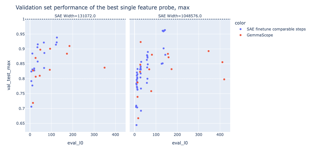

Initially, we expected that SAE based probes would not outperform linear probes on in-distribution data, but we expected that they might have an advantage out of distribution, especially those based on a single feature or a small number of features, under the hypothesis that SAE features would generalise more robustly out of distribution. However, we generally find that even on the OOD set, SAE probing does not match the performance of a linear probe, though the best single feature probe from the finetuned model does come close in some cases. We were surprised by the performance and robustness of the linear probe, and this is consistent with probes beating SAEs in OOD settings studied by Kantamneni et al, though we can’t make confident extrapolations about probes vs SAEs in all OOD settings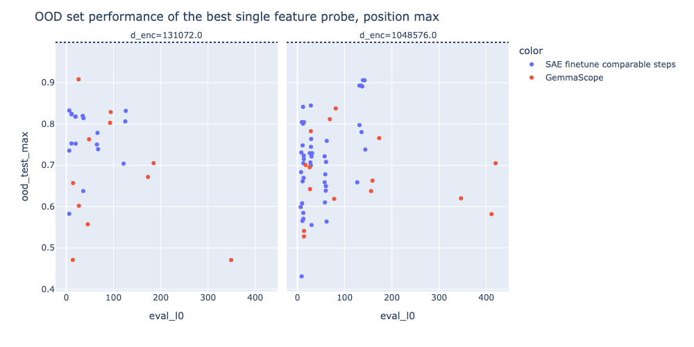

We can expand on single feature probes by using k-sparse probing, for k between 2 and 50. Using k-sparse probing largely closes the gap to the near-perfect performance dense probes for K>=5, although generally a small gap remains. Notably, despite k-sparse probing performing near perfectly in distribution, it shows worse transfer OOD, while dense probes generalise well, the opposite of what we predicted should happen with high quality SAEsl.

We experiment with two methods for k-sparse probing; selecting k latents by sorting by the mean difference of latent activations between positive and negative examples in the training set, and using l1 regression with a coefficient swept to select a number of active probe latents close to the target k (and then retraining an unregularised model on the selected latents). The two methods generally show similar results, as shown below, matching the results of Gurnee et al on neurons.

Our results with k-sparse probing generally corroborate our results that finetuning SAEs helps, with finetuned SAEs generally outperforming the original GemmaScope SAEs, particularly for low L0 values, but it is not enough to achieve parity with dense probes.

Related Work and Discussion

SAE probing was also studied in parallel by Kantamneni et al and Bricken et al. Generally, we think that our results are fairly consistent with the literature here. In particular, Kantamneni et. al. try to carry out a similar analysis to us over a wide variety of datasets, finding broadly comparable results to us; that sparse probing wins only rarely, having an advantage only when the labels are highly corrupted or potentially in low-data regimes. They also found better performance on simpler datasets where the SAE had a single highly relevant latent, and not on more subtle datasets.

Similarly, Bricken et al recently studied how SAE probes compare to linear probes. They study detecting biology-related misuse, rather than harmful intent. Unlike us, they find a slight advantage for SAEs in that SAEs allow max-aggregating latents along the sequence dimension before training a classifier (max-pooling the activations), which lets their classifier be more sensitive to data distributed throughout the prompt. Though Kantamneni et al show that, though max-aggregating latents can be an advantage over single token dense probes in some settings, it does not systematically beat attention head probes, and we speculate that attention head probes would also do well in our setting. We do not find that max-pooling is particularly helpful for our task ; we hypothesise that this may be because the information relevant to the classifier in our case is fairly temporally concentrated.

Like us, both Kantamneni et al and Bricken et al find that the individual SAE latents are useful for finding spurious correlations in a dataset. Notably, Kantamneni et al find a single latent predicting grammatical accuracy, with similar accuracy to the “ground truth” labels in Glue CoLA, due to the high level of label noise. In some ways, our empirical results understate the utility of this, as we used the inspectability of our probes in order to clean our datasets of spurious correlations; if we hadn’t done this, our linear probes would presumably have learnt these too, which would have decreased their generalisation out of distribution. However, Kantamneni et al showed that these spurious correlations could be discovered by other methods, which we speculate would work for us too.

In general, we do find that there is a persistent performance gap between SAEs and probes. In part, this is because SAEs remain imperfect, and we do find that relevant information is lost in the reconstruction term, with probes on the SAE reconstruction generally performing slightly worse than a probe on the raw residual stream.

Performance delta between probe trained on residual stream and on SAE reconstruction.

Consistent with these negative results for SAE probing, very recent work by Apollo Research also tried SAE probes for detecting deceptive behaviour, finding that linear probes outperformed SAE probing.

We think it is curious that many of the variations on finetuning we tried did not seem to make a significant difference. It is possible that our setup is very noisy; perhaps a larger probing dataset would allow us to see a significant difference between these methods.

Is it surprising that SAEs didn’t work?

In general, we found it unexpectedly hard to reason about how to update from positive/negative results on downstream tasks. In some sense, we have a hammer and are looking for a nail. We have this cool technique of SAEs, and want to find problems well suited to it. We care about how often it’s useful, and the magnitude of benefit. It doesn’t need to be useful for everything, but we care much more about some tasks than others. If you find one successful application, that doesn’t mean it will work in less cherry-picked cases, and if you have one failure, maybe it was badly suited to SAEs, but other important tasks would work fine. And even if you do have several successes, that may not be enough to justify the costs of training and R&D. Overall, we think that seeking evidence of interpretability on downstream tasks is valuable and something we hope to see more of in future - you can’t update too much off of the evidence, but it seems like a crucial question and this is one of the better sources of evidence we can currently access.

Another complication is that interpretability is quite hard to reason clearly about in general. You might have success on a task, but for quite different reasons than you thought, and you might think SAEs should help on a task, but actually your intuition is wrong. To illustrate this, in hindsight, we're now a lot more confused about whether even an optimal SAE should beat linear probes on OOD generalisation.

Here’s our fuzzy intuition for what’s going on. We have a starting distribution, an OOD distribution, a train set and a val set (from the original distribution) and an OOD test set. There are three kinds of things a probe can learn for predicting the train set:

1. Noise: patterns specific to the train set that do not generalise out of sample, i.e. on the test set. Learning noise gives rise to overfitting.
2. Spurious correlations: patterns that predict the concept in the original distribution (and which are predictive even on the test set) but that do not generalise out of distribution.
3. True signal: patterns that are predictive of the target concept both in-distribution and out-of-distribution.

Noise is easily ignored given enough data. Indeed, on this task we found that both SAEs and linear probes learn to basically classify perfectly on the test set (i.e. out of sample, but in-distribution). So the difference in performance between SAEs and linear probes out of distribution comes down to how their respective inductive biases help them to latch on to the true signal versus spurious correlations: it seems that SAE probes do a worse job at this than linear probes. Why is this?

Our original hypothesis had been that sparse SAE probes would in fact have a better inductive bias for picking the true signal over spurious correlations. This was in large part because we had assumed that the concept we’re looking to learn (“harmful intent”) is a fairly simple logical expression, composed of a small number of “atomic” concepts, both causal (like danger, violence, profanity, etc) and correlational (like linguistic features indicative of users who are trying to commit harm or of jailbreaks), that we expected SAEs would have assigned to single / small clusters of latents. Under this assumption, we guessed that a sparse SAE probe would easily find the relevant concepts among its latents and therefore extract the true signal, ignore spurious correlations. The fact that this doesn’t happen suggests a number of things that could be going wrong:

1. The concept “harmful intent” (as defined implicitly by the harmful datasets we used to train the probe) may not really be a simple function of a few “atomic” concepts at all. I.e., even with an “perfect” SAE - one whose latents correspond precisely to the concepts the model uses - it could be the case that the positive and negative labels in our datasets can’t be generated by a simple expression involving just a few of these concepts.
   1. This could indicate a fundamental problem with SAEs - we want concepts like harmful intent, and if high functioning SAEs do not usefully isolate them, this is bad
   2. Or it could just be that harmful intent is a fuzzily defined concept, and depends a lot on the subjective values of the labellers/those setting rules for labellers. Though under this hypothesis, it’s surprising that linear probes generalise well.
2. Even if “harmful intent” is really a simple function of a few basic interpretable concepts, because our SAEs don’t learn these concepts cleanly, a sparse SAE probe doesn’t manage to capture the true signal.
3. Since SAEs are incomplete, perhaps important directions corresponding to components of the true signal are missing from the dictionary, forcing the SAE probe to make do with approximating these directions from the latents that it does possess.
4. Patterns that are spurious correlations may be just as well represented by latents in the SAE’s dictionary as patterns that make up the true signal, meaning that there is no reason to expect a sparse SAE probe to preferentially latch onto components of the true signal over spurious correlations.

In practice, our guess is that a mix of these are going on. b and c would suggest that we just haven’t gotten good enough at training SAEs but that it may be a promising direction, and a suggests fundamental issues with SAEs as a method. d would suggest that SAEs could make a promising probing method if we augmented them by pruning out latents that seemed like spurious correlations, but we de facto already did this by using them to clean up correlations in the data itself benefitting both the SAE probe and the dense probe. Overall, this means that it’s hard to draw a clear conclusion from the data available, but it does seem a bad sign for the practical utility of SAEs.

Dataset debugging with SAEs

Sen Rajamanoharan, Lewis Smith, Arthur Conmy

One use case where we did find SAEs useful was in dataset debugging. As the SAE latents are (somewhat) interpretable, inspecting the latents with big mean differences between positive and negative labels can reveal useful information about our dataset. This mirrors similar findings in Kantamneni et al and Bricken et al

For instance, when running an early version of this, when inspecting the best performing features at separating Alpaca and HarmBench, we realised that one of the best performing was a feature that seemed to be a question mark feature. On inspection, we realised that only Alpaca contained questions, whereas the harmful examples were all instructions. Being able to inspect the dataset in this way using a model with SAEs was definitely useful in catching this error, and other than manual inspection, it’s not clear if we ever would have noticed this if we exclusively used linear probing. Though Kantamneni et al were able to achieve similar results by taking maximum activating dataset examples of a linear probe over the pretraining data.

This also somewhat complicates the story that linear probing generally performed better than SAEs; this is presumably partly because we were able to use SAEs to manually clean spurious correlations from our dataset before training a supervised probe.

One interesting thing to note here is that you can use SAE based techniques like this for dataset exploration even if you don’t have an SAE on the model you want to probe on; for instance, using a model like Gemma 2 with an SAE sweep could be used to try to detect issues like this before you train something based on a larger model, as we are interested in the properties of the data, not the model.

This exploratory property is one reason why people expect that unsupervised techniques like SAEs will be useful for safety work; as they make it easier to discover unanticipated features of the model than supervised techniques. However, as mentioned, in this instance SAEs have seemed primarily useful as a technique for investigating datasets as much as models.

Autointerp and high frequency latents

Callum McDougall

In the next section, we’ll compare autointerpretability scores across models with different latent density distributions (in particular, some models with more high-frequency features than others). This introduces a problem - traditionally autointerp is measured as an average score over all latents, but this doesn’t capture the fact that eliminating a high-frequency uninterpretable feature is intuitively better than eliminating a low-frequency uninterpretable feature. One way to think about this is, if we sampled a prompt from the pretraining distribution and gave it to the model, and look at the latents, we’d hope that they tend to be interpretability. But the correct way to measure this is by taking the autointerp score for each latent weighted by how frequent they are, not uniformly weighted. We have found taking frequency weighted auto-interp scores to be instructive, and recommend that practitioners plot this, in addition to uniform weighted.

As an extreme example, we can construct a pathological SAE where 𝑀−𝑁 latents encode specific bigrams and the remaining 𝑁 latents fully reconstruct the rest of the 𝑁-dimensional SAE input - this would score very well on autointerp with uniform average scores provided 𝑀 >> 𝑁, but poorly with frequency-weighted average scores. For this reason, although we show both uniform and frequency-weighted autointerp results in the experiments below, we’ll focus more on the frequency-weighted scores in subsequent discussion.

Aside from this weighting strategy, the rest of the autointerp methodology follows standard practices such as those introduced in Bills et al and built on by EleutherAI. An explanation is generated by constructing a prompt that contains top activating example sequences as well as examples sampled from each quantile and a selection of random non-activating examples, and asking the model to characterise the kinds of text which causes the latent to fire. We then give the model a set of unlabelled sequences (some from the top activaing or quantile groups, others non-activating) and ask it to estimate the quantised activation value of the highest-activating token in that sequence. The latent’s interpretability score is then computed as the spearman correlation between the true estimated quantised activations.

Removing High Frequency Latents from JumpReLU SAEs

Senthooran Rajamanoharan, Callum McDougall, Lewis Smith

TL;DR: Both JumpReLU and TopK SAEs suffer from high frequency latents: latents that fire on many tokens ($>10\%$ of the dataset) and often seem uninterpretable. We find that by tweaking the sparsity penalty used to train JumpReLU SAEs we can largely eliminate high frequency latents, with only a small cost in terms of reconstruction error at fixed L0. Auto-interp suggests that this has a neutral-to-positive effect on the average latent interpretability once we weight by latent frequency, by reducing the incidence of high frequency uninterpretable latents.

Method

Motivation

In our paper, we trained JumpReLU SAEs using a L0 sparsity penalty, which penalises a SAE in proportion to the number of latents that fire on each token:

Where $f_i\left(x_{\alpha }\right)$ is the activation of the $i^{th}$ latent on an $N$-dimensional input LM activation $x$, and $M$ is the width (total number of latents) of the SAE.^[1]

This L0 sparsity penalty only cares about controlling the average firing frequency across all latents in a SAE; it is actually indifferent to the range of firing frequencies in the SAE. In other words, L0 doesn’t care whether a low firing frequency is achieved by: (a) all latents firing infrequently, or (b) some latents firing frequently and other latents firing very infrequently to compensate. As long as the average firing frequency is the same either way, L0 doesn’t mind.^[2]

We can see this formally, by noticing that the average L0 penalty on a training batch can be expressed as follows:

where ${\hat{\omega }}_i:=\frac{1}{B}{\sum }_{\alpha =1}^B{1}_{f_i\left(x_{\alpha }\right)>0}$ is a single-batch estimate of the firing frequency of the $i^{th}$latent and $⟨\hat{\omega }⟩$ is the mean firing frequency (as estimated on this batch) across all latents in the SAE. Hence, the L0 sparsity penalty is exactly proportional to the mean of the SAE’s firing frequency histogram, and therefore indifferent to the spread of latent firing frequencies in this histogram. This in turn leads to the rise of high frequency latents: as long as these latents are beneficial for minimizing the SAE's reconstruction error, training with a L0 penalty provides insufficient pressure to prevent high frequency latents from forming, as can be seen following frequency histograms.

Modifying the sparsity penalty

Now, a nice feature of JumpReLU SAEs is that we are not beholden to using a L0 sparsity penalty.^[3] Given the observation above, an obvious way to get rid of high frequency features is modify the sparsity penalty so that it does penalise dispersion (and in particular right-tail dispersion) in addition to the mean of the firing frequency histogram. There are many ways to do this, but here we explore arguably the simplest approaches to achieving this property, which is to add a term to the sparsity penalty that is quadratic in latent frequencies:

Note that the first term in this quadratic-frequency sparsity penalty is the standard L0 penalty, whereas the second term is proportional to the mean squared latent frequency. We have introduced a new hyperparameter ${\omega }_0$, which sets the frequency scale at which the sparsity penalty switches from penalising latent frequency roughly linearly (for latents with frequencies ${\hat{\omega }}_i\ll {\omega }_0$), to penalising latent frequency quadratically (for latents with frequencies ${\hat{\omega }}_i\gtrsim {\omega }_0$). This in turn leads to this penalty disincentivising high frequency latents from appearing, while latents lower down the frequency distribution are treated similarly to latents in a standard (L0-based) JumpReLU SAE.^[4]

How we evaluated interpretability

When evaluating the effectiveness of JumpReLU variants, we face a problem: traditionally the interpretability of a SAE is measured as the average auto-interp score over all its latents, but this doesn't capture the fact that eliminating a high-frequency uninterpretable latent is typically better than eliminating a low-frequency uninterpretable latent. As an extreme example, we can construct a pathological SAE where $M-N$latents encode specific bigrams and the remaining $N$ latents fully reconstruct the rest of the $N$-dimensional SAE input: this would score very well on auto-interp with uniform average scores provided $M\gg N$, but poorly with frequency-weighted average scores. For this reason, although we show both uniform and frequency-weighted auto-interp results in the experiments below, we'll focus more on the frequency-weighted scores in the subsequent discussion.^[5]

Aside from this weighting strategy, the rest of the auto-interp methodology follows standard practices such as those introduced in Bills et al. (2023) and built on by Paulo et al. (2024). An explanation is generated by constructing a prompt that contains top activating example sequences as well as examples sampled from each quantile and a selection of random non-activating examples, and asking the model to characterise the kinds of text which causes the latent to fire. We then give the model a set of unlabelled sequences (some from the top activating or quantile groups, others non-activating) and ask it to estimate the quantised activation value of the highest-activating token in that sequence. The latent's interpretability score is then computed as the Spearman correlation between the true & estimated quantised activations.

Results

In our experiments below, we try setting the frequency scale ${\omega }_0$ to either ${10}^{-1}$ or ${10}^{-2}$, since we are interested in suppressing latents that fire on more than about 10% of tokens. We compare quadratic-frequency loss JumpReLU SAEs trained this way against standard (L0 penalty) JumpReLU SAEs, Gated SAEs and TopK SAEs.^[6] We train 131k SAEs from scratch on layer 20 Gemma 2 9B IT activations on instruction tuning data [TODO: reference back to a description of this from an earlier snippet].

Reconstruction loss at fixed sparsity

As expected (since we are no longer optimising for L0 directly), JumpReLU SAEs trained with the quadratic-frequency penalty have slightly worse reconstruction loss at a given sparsity than JumpReLU SAEs trained with the standard L0 loss. However, the quadratic-frequency penalty JumpReLU SAEs still compare favourably to TopK and Gated SAEs.

Frequency histograms

As shown above, the quadratic-frequency penalty successfully suppresses high-frequency latents without having a noticeable effect on the shape of the remainder of the frequency histogram (particularly in the case ${\omega }_0={10}^{-1}$).

Latent interpretability

As shown above, we observe that the uniform average scores don't show a clear pattern (with Gated & TopK SAEs slightly outperforming for given sparsity values, and JumpReLU variants slightly under-performing). But the frequency-weighted plots show much clearer patterns: (1) nearly all SAEs have lower average latent interpretability scores at larger L0 values (which makes sense under the hypothesis that penalizing lack of sparsity leads to more monosemantic latents), and (2) the JumpReLU variants go against this trend for high L0 values by actually getting more interpretable. Digging deeper into this, we can plot the average latent auto-interp score for each SAE at different latent frequency quantiles, as shown in the appendix [TODO: LINK], for the standard JumpReLU and the quadratic-frequency loss variant with $\omega =0.01$. We find that SAEs at all sparsity levels show a negative trend of latent interpretability against latent frequency, although the quadratic-frequency variant still has high-frequency and interpretable latents at all sparsity levels.

Conclusions

In this snippet we've shown how it's possible to modify the JumpReLU loss function to obtain further desirable properties, like removing high frequency latents.

The quadratic-frequency penalty successfully eliminates high frequency latents with only a modest impact on reconstruction loss at fixed sparsity. On auto-interp it tends to score better than standard JumpReLU when we weight individual latents' interpretability scores by frequency (which penalises uninterpretable high frequency latents more heavily than uniform weighting), although at lower L0s Gated SAEs seem to have the best scores of all the SAE varieties we evaluated. Counter-intuitively (and in contrast to the other SAE varieties), the average interpretability of quadratic-frequency SAEs seems to increase with L0 beyond a certain point! We don't have a good explanation for this phenomenon and haven't investigated it further.

Does this mean the quadratic-frequency penalty is an improvement over standard JumpReLU SAEs trained with a L0 penalty? We're unsure for a number of reasons:

• We haven't evaluated these variants extensively, for example on downstream tasks like steering or probing.
• It's unclear whether we should really aim to remove high frequency latents in the first place. Perhaps they do represent meaningful directions in activation space that we just haven't been able to interpret yet. It's also possible that some high frequency features are pathological and others are legitimate, and we need a more nuanced loss than simply penalising firing frequency to target the former without affecting the latter.
• The quadratic-frequency loss may simply promote partitioning individual high frequency latents into several (similarly uninterpretable) lower frequency latents, effectively sweeping the problem under the rug.^[7]
• We haven't tried stacking these changes with other improvements like a Matryoshka reconstruction loss (to deal with feature absorption) or the ideas in Anthropic's January 2025 update.

Nevertheless, by sharing our ideas and results, we hope that practitioners who run into issues with high frequency latents may try variants on the standard JumpReLU loss like quadratic-frequency (or iterate further on them) and see if they provide an improvement for their use case.

Appendix

1. ^{^}

   As we describe in detail in the paper, we use straight-through-estimators (STEs) to differentiate through the step discontinuities in both the L0 sparsity penalty and the jump discontinuity in the JumpReLU activation function to train JumpReLU SAEs. We use the same method here.

2. ^{^}

   A very similar argument can be made about TopK SAEs, which control L0 via the $k$ parameter.

3. ^{^}

   Indeed, in our paper, we show how we can modify the sparsity penalty to train SAEs that target a fixed L0, much like TopK SAEs. Here, we will instead modify the sparsity penalty to directly target high frequency features. 

4. ^{^}

   An alternative, and even simpler, sparsity penalty would be to penalise all latents according to the square of their firing frequencies, i.e. using a penalty of the form $\lambda {\sum }_{i=1}^M{\hat{\omega }}_i^2$. This squared-frequency penalty also has the advantage of not introducing yet another hyperparameter. However, this penalty under-penalises latents with very low firing frequencies, leading to a frequency distribution that is devoid of both high and low firing frequencies, i.e. more sharply peaked around the mean firing frequency. One way to see why this is the case is to notice that such a penalty can also be expressed as $⟨\hat{\omega }{⟩}^2+Var\left(\omega \right)$: i.e. holding the mean firing frequency $⟨\hat{\omega }⟩$ fixed, it corresponds to minimising the variance of the frequency distribution. In contrast, the quadratic-frequency sparsity penalty here ensures that all latents receive a frequency penalty that is at least linear, while high frequency latents receive an additional penalty that is quadratic; this ensures that the lower part of the frequency distribution remains similar to the latent frequency distributions for JumpReLU and TopK, while nevertheless suppressing the top end of the frequency distribution.

5. ^{^}

   Note that this is a departure from the approach we've taken in earlier work, where latents were sampled for auto/manual auto-interp uniformly and with a low-frequency cutoff to deal with latents that have insufficient data.

6. ^{^}

   We train all JumpReLU variants using straight-through-estimators that only provide gradients to the threshold, as in the original paper.

7. ^{^}

   This could be happening with Gated SAEs too.