In this post, we’re going to use the diagrammatic notation of Bayes nets. However, we use the diagrams a little bit differently than is typical. In practice, such diagrams are usually used to define a distribution - e.g. the stock example diagram

... in combination with the five distributions $P\left[\text{Season}\right]$, $P\left[\text{Rain}|\text{Season}\right]$, $P\left[\text{Sprinkler}|\text{Season}\right]$, $P[\text{Wet}|\text{Rain},\text{Sprinkler}]$, $P\left[\text{Slippery}|\text{Wet}\right]$, defines a joint distribution

$P[\text{Season},\text{Rain},\text{Sprinkler},\text{Wet},\text{Slippery}]$

$=P\left[\text{Season}\right]P\left[\text{Rain}|\text{Season}\right]P\left[\text{Sprinkler}|\text{Season}\right]P[\text{Wet}|\text{Rain},\text{Sprinkler}]P\left[\text{Slippery}|\text{Wet}\right]$

In this post, we instead take the joint distribution as given, and use the diagrams to concisely state properties of the distribution. For instance, we say that a distribution $P[\Lambda ,X]$ “satisfies” the diagram

if-and-only-if $P[\Lambda ,X]=P\left[\Lambda \right]{\prod }_{i}P\left[X_i|\Lambda \right]$. (And once we get to approximation, we’ll say that $P[\Lambda ,X]$ approximately satisfies the diagram, to within $ϵ$, if-and-only-if $D_{KL}\left(P\right[\Lambda ,X\left]||P\right[\Lambda \left]{\prod }_{i}P\right[X_i|\Lambda \left]\right)\le ϵ$.)

The usage we’re interested in looks like:

• State that some random variables satisfy several different diagrams
• Derive some new diagrams which they satisfy

In other words, we want to write proofs diagrammatically - i.e. each “step” of the proof combines some diagrams (which the underlying distribution satisfies) to derive a new diagram (which the underlying distribution satisfies).

For this purpose, it’s useful to have a few rules for an “algebra of diagrams”, to avoid always having to write out the underlying factorizations in order to prove anything. We’ll walk through a few rules, give some examples using them, and prove them in the appendix. The rules:

• Re-Rooting Rule for Markov Chains
• Joint Independence Rule
• Frankenstein Rule
• Factorization Transfer Rule
• Stitching Rule for A Shared Markov Blanket
• Bookkeeping Rules

The first couple are relatively-simple rules for “serial” and “parallel” variables, respectively; they’re mostly intended to demonstrate the framework we’re using. The next four rules are more general, and give a useful foundation for application. Finally, the Bookkeeping Rules cover some “obvious” minor rules, which basically say that all the usual things we can deduce from a single Bayes net still apply.

Besides easy-to-read proofs, another big benefit of deriving things via such diagrams is that we can automatically extend our proofs to handle approximation (i.e. cases where the underlying distribution only approximately satisfies the diagrams). We’ll cover approximate versions of the rules along the way.

Finally, we’ll walk through an end-to-end example of a proof which uses the rules.

Re-Rooting Rule for Markov Chains

Suppose we have a distribution over $X_1,X_2,X_3,X_4$ which satisfies

Then the distribution also satisfies all of these diagrams:

In fact, we can also go the other way: any one of the above diagrams implies all of the others.

Since this is our first rule, let’s unpack all of that compact notation into its full long-form, in a concrete example. If you want to see the proof, take a look at the appendix.

Verbose Example

For concreteness, let’s say we have a widget being produced on an assembly line. No assembly line is perfect; sometimes errors are introduced at a step, like e.g. a hole isn’t drilled in quite the right spot. Those errors can then cause further errors in subsequent steps, like e.g. the hole isn’t in quite the right spot, a part doesn’t quite fit right. We’ll say that $X_1$ is the state of the widget after step 1, $X_2$ is the state after step 2, etc; the variables are random to model the “random” errors sometimes introduced.

Our first diagram

says that the probability of an error at step $i$, given all the earlier steps, depends only on the errors accumulated up through step $i-1$. That means we’re ignoring things like e.g. a day of intermittent electrical outages changing the probability of error in every step in a correlated way. Mathematically, we get that interpretation by first applying the chain rule (which applies to any distribution) to the underlying distribution:

$P[X_1,X_2,X_3,X_4]=P\left[X_1\right]P\left[X_2|X_1\right]P[X_3|X_2,X_1]P[X_4|X_3,X_2,X_1]$

(we can also think of the chain rule as a “universal diagram” satisfied by all distributions; it’s a DAG with an edge between every two variables). We then separately write out the factorization stated by the diagram:

$P[X_1,X_2,X_3,X_4]=P\left[X_1\right]P\left[X_2|X_1\right]P\left[X_3|X_2\right]P\left[X_4|X_3\right]$

Equating these two (then marginalizing variables different ways and doing some ordinary algebra), we find:

• $P\left[X_1\right]=P\left[X_1\right]$ (duh)
• $P\left[X_2|X_1\right]=P\left[X_2|X_1\right]$ (also duh)
• $P[X_3|X_2,X_1]=P\left[X_3|X_2\right]$
• $P[X_4|X_3,X_2,X_1]=P\left[X_4|X_3\right]$

… which we can interpret as “probability of an error at step $i$, given all the earlier steps” - i.e. the left-hand side of each of the above - “depends only on the errors accumulated up through step $i-1$” - i.e. the right-hand side of each of the above. (Note: many of the proofs for rules in this post start by "breaking things up" this way, using the chain rule.)

So far, we’ve just stated what the starting diagram means. Now let’s look at one of the other diagrams:

The factorization stated by this diagram is

$P[X_1,X_2,X_3,X_4]=P\left[X_1|X_2\right]P\left[X_2|X_3\right]P\left[X_3\right]P\left[X_4|X_3\right]$

Interpretation: we could model the system as though the error-cascade “starts” at step 3, and then errors propagate back through time to steps 2 and 1, and forward to step 4. Obviously this doesn’t match physical causality (i.e. do() operations will give different results on the two diagrams). But for purposes of modeling the underlying distribution $P[X_1,X_2,X_3,X_4]$, this diagram is equivalent to the first diagram.

What does “equivalent” mean here? It means that any distribution which satisfies the factorization expressed by the first diagram (i.e. $P[X_1,X_2,X_3,X_4]=P\left[X_1\right]P\left[X_2|X_1\right]P\left[X_3|X_2\right]P\left[X_4|X_3\right]$) also satisfies the factorization expressed by the second diagram (i.e. $P[X_1,X_2,X_3,X_4]=P\left[X_1|X_2\right]P\left[X_2|X_3\right]P\left[X_3\right]P\left[X_4|X_3\right]$), and vice versa.

More generally, this is a standard example of what we mean when we say “diagram 1 implies diagram 2”, for any two diagrams: it means that any distribution which satisfies the factorization expressed by diagram 1 also satisfies the factorization expressed by diagram 2. If the two diagrams imply each other, then they are equivalent: they give us the same information about the underlying distribution.

Back to the example: how on earth would one model the widget error-cascade as starting at step 3? Think of it like this: if we want to simulate the error-cascade (i.e. write a program to sample from $P[X_1,X_2,X_3,X_4]$), we could do that by:

• First sampling $X_3$
• … then working backward to the distribution of $X_2$ given that $X_3$ value, and sampling $X_2$ from that distribution
• … then further back from $X_2$ to $X_1$
• … and on the other side, sampling $X_4$ from $X_3$

When we frame it that way, it’s not really something physical which is (modeled as) propagating back through time. Rather, we’re just epistemically working backward as a way to “solve for” the system’s behavior. And that’s a totally valid way to “solve for” this system’s behavior (though I wouldn’t personally want to code it that way).

In the context of our widget example, this seems… not very useful. Sure, the underlying distribution can be modeled using some awkward alternative diagram, but the alternative diagram doesn’t really seem better than the more-intuitive starting diagram. More generally, our rule for re-rooting Markov Chains is usually useful as an intermediate in a longer derivation; the real value isn’t in using it as a standalone rule.

Re-Rooting Rule, More Generally

More generally, any diagram of the form

is equivalent to any other diagram of the same form (i.e. take any other “root node” $i$).

For approximation, if the underlying distribution approximately satisfies any diagram of the form

to within $ϵ$, then it satisfies all the others to within $ϵ$.

Again, since this is our first rule, let’s unpack that compact notation. The diagram

expresses the factorization

$P[X_1,\dots ,X_n]=\left({\prod }_{i\le k}P\right[X_{i-1}|X_i\left]\right)P\left[X_k\right]\left({\prod }_{k\le i\le n-1}P\right[X_{i+1}|X_i\left]\right)$

We say that the underlying distribution $P[X_1,\dots ,X_n]$ “approximately satisfies the diagram to within $ϵ$” if-and-only-if

$D_{KL}\left(P\right[X_1,\dots ,X_n\left]||\right({\prod }_{i\le k}P\left[X_{i-1}|X_i\right]\left)P\right[X_k\left]\right({\prod }_{k\le i\le n-1}P\left[X_{i+1}|X_i\right]\left)\right)\le ϵ$

So, our approximation claim is saying: if $D_{KL}\left(P\right[X_1,\dots ,X_n\left]||\right({\prod }_{i\le k}P\left[X_{i-1}|X_i\right]\left)P\right[X_k\left]\right({\prod }_{k\le i\le n-1}P\left[X_{i+1}|X_i\right]\left)\right)\le ϵ$ for any $i$, then $D_{KL}\left(P\right[X_1,\dots ,X_n\left]||\right({\prod }_{i\le k}P\left[X_{i-1}|X_i\right]\left)P\right[X_k\left]\right({\prod }_{k\le i\le n-1}P\left[X_{i+1}|X_i\right]\left)\right)\le ϵ$ for all $i$. Indeed, the proof (in the appendix) shows that those $D_{KL}$’s are all equal.

Joint Independence Rule

Suppose I roll three dice $(X_1,X_2,X_3)$. The first roll, $X_1$, is independent of the second two, $(X_2,X_3)$. The second roll, $X_2$, is independent of $(X_1,X_3)$. And the third roll, X_3, is independent of $(X_1,X_2)$. Then: all three are independent.

If you’re like “wait, isn’t that just true by definition of independence?”, then you have roughly the right idea! (Some-but-not-all sources define many-variable independence this way.) But if we write out the underlying diagrams/math, it will be more clear that we have a nontrivial (though simple) claim. Our preconditions say:

or, in standard notation

$P[X_1,X_2,X_3]=P\left[X_1\right]P[X_2,X_3]$

$P[X_1,X_2,X_3]=P\left[X_2\right]P[X_1,X_3]$

$P[X_1,X_2,X_3]=P\left[X_3\right]P[X_1,X_2]$

Our claim is that these preconditions together imply:

or in the usual notation

$P[X_1,X_2,X_3]=P\left[X_1\right]P\left[X_2\right]P\left[X_3\right]$

That’s pretty easy to prove, but the more interesting part is approximation. If our three diagrams hold to within ${ϵ}_1,{ϵ}_2,{ϵ}_3$ respectively, then the final diagram holds to within ${ϵ}_1+{ϵ}_2+{ϵ}_3$. Writing it out the long way:

$D_{KL}\left(P\right[X_1,X_2,X_3\left]||P\right[X_1\left]P\right[X_2,X_3\left]\right)\le {ϵ}_1$

$D_{KL}\left(P\right[X_1,X_2,X_3\left]||P\right[X_2\left]P\right[X_1,X_3\left]\right)\le {ϵ}_2$

$D_{KL}\left(P\right[X_1,X_2,X_3\left]||P\right[X_3\left]P\right[X_1,X_2\left]\right)\le {ϵ}_3$

(Note that, in the dice example, these $D_{KL}$’s are each the mutual information of one die with the others, since $MI(X;Y)=D_{KL}\left(P\right[X,Y\left]||P\right[X\left]P\right[Y\left]\right)$ in general.) Together, they imply:

$D_{KL}\left(P\right[X_1,X_2,X_3\left]||P\right[X_1\left]P\right[X_2\left]P\right[X_3\left]\right)\le {ϵ}_1+{ϵ}_2+{ϵ}_3$

In the context of the dice example: if I think that each die $i$ individually is approximately independent of the others (to within ${ϵ}_i$ bits of mutual information), that means the dice are all approximately jointly independent (to within ${\sum }_i{ϵ}_i$ bits).

More generally, this all extends in the obvious way to more variables. If I have $n$ variables, each of which is individually independent of all the others, then they’re all jointly independent. In the approximate case, if each of variables $X_1\dots X_n$ has only mutual information ${ϵ}_i$ bits with the others, then the variables are jointly independent to within ${\sum }_i{ϵ}_i$ bits - i.e.

$D_{KL}\left(P\right[X\left]||{\prod }_{i}P\right[X_i\left]\right)\le {\sum }_i{ϵ}_i$

We can also easily extend the rule to conditional independence: if each of the variables $X_1\dots X_n$ has mutual information at most ${ϵ}_i$ with the others conditional on some other variable $Y$, then the variables are jointly independent to within ${\sum }_i{ϵ}_i$ bits conditional on $Y$. Diagrammatically:

The Frankenstein Rule

Now on to a more general/powerful rule.

Suppose we have an underlying distribution $P[X_1\dots X_5]$ which satisfies both of these diagrams:

Notice that we can order the variables $(X_1,X_3,X_2,X_5,X_4)$; with that ordering, there are no arrows from “later” to “earlier” variables in either diagram. (We say that the ordering “respects both diagrams”.) That’s the key precondition we need in order to apply the Frankenstein Rule.

Because we have an ordering which respects both diagrams, we can construct "Frankenstein diagrams", which combine the two original diagrams. For each variable, we can choose which of the two original diagrams to take that variable’s incoming arrows from. For instance, in this case, we could choose:

• Incoming arrows of $X_1$ from the left diagram
• Incoming arrows of $X_3$ from the right diagram
• Incoming arrows of $X_2$ from the left diagram
• Incoming arrows of $X_5$ from the left diagram
• Incoming arrows of $X_4$ from the left diagram

resulting in this diagram:

But we could make other choices instead! We could just as easily choose:

• Incoming arrows of $X_1$ from the right diagram
• Incoming arrows of $X_3$ from the left diagram
• Incoming arrows of $X_2$ from the right diagram
• Incoming arrows of $X_5$ from the right diagram
• Incoming arrows of $X_4$ from the left diagram

which would yield this diagram:

The Frankenstein rule says that, so long as our underlying distribution satisfies both of the original diagrams, it satisfies any Frankenstein of the original diagrams (so long as there exists an order of the variables which respects both original diagrams).

More generally, suppose that:

• Our underlying distribution $P[X_1,\dots ,X_n]$ satisfies two different diagrams, and
• There exists some ordering of the variables $X_1\dots X_n$ which respects the order of both diagrams simultaneously (i.e. when the variables are in that order, there’s never an arrow from a “later” variable to an “earlier” variable in either diagram).

If those two conditions hold, then we can create an arbitrary “Frankenstein diagram” from the two original diagrams: for each variable, we can take its incoming arrows from either of the two original diagrams. The underlying distribution will satisfy any Frankenstein diagram.

We can also extend the Frankenstein Rule to more than two original diagrams in the obvious way: so long as there exists an ordering of the variables which respects all diagrams, we can construct a Frankenstein which takes the incoming arrows of each variable from any of the original diagrams.

For approximation, we have two options. One approximate Frankenstein rule is simpler but gives mildly looser bounds, the other is a little more complicated but gives mildly tighter bounds (especially as the number of original diagrams increases).

The simpler approximation rule: if the original two diagrams are satisfied to within ${ϵ}_1$ and ${ϵ}_2$, respectively, then the Frankenstein is satisfied to within ${ϵ}_1+{ϵ}_2$. (And this extends in the obvious way to more-than-two original diagrams.)

The more complex approximation rule requires some additional machinery. For any diagram, we can decompose its $D_{KL}$ into one term for each variable via the chain rule:

$D_{KL}\left(P\right[X_1,\dots ,X_n\left]||{\prod }_{i}P\right[X_i|X_{pa\left(i\right)}\left]\right)=D_{KL}\left({\prod }_{i}P\right[X_i|X_{<i}\left]||{\prod }_{i}P\right[X_i|X_{pa\left(i\right)}\left]\right)$

$={\sum }_{i}E\left[D_{KL}\right(P\left[X_i|X_{<i}\right]||P\left[X_i|X_{pa\left(i\right)}\right]\left)\right]$

If we know how our upper bound $ϵ$ on the diagram’s $D_{KL}$ decomposes across variables, then we can use that for more fine-grained bounds. Suppose that, for each diagram $j$ and variable $i$, we have an upper bound

${ϵ}_j^i\ge E\left[D_{KL}\right(P\left[X_i|X_{<i}\right]||P\left[X_i|X_{p{a}_j\left(i\right)}\right]\left)\right]$

Then, we can get a fine-grained bound for the Frankenstein diagram. For each variable $i$, we add only the ${ϵ}_j^i$ from the original diagram $j$ from which we take that variables’ incoming arrows to build the Frankenstein. (Our simple approximation rule earlier added together all the ${ϵ}_j^i$’s from all of the original diagrams, so it was over-counting.)

Exercise: Using the Frankenstein Rule on the two diagrams at the beginning of this section, show that $X_3$ is independent of all the other variables (assuming the two diagrams from the beginning of this section hold).

Factorization Transfer Rule

The factorization transfer rule is of interest basically-only in the approximate case; the exact version is quite trivial.

Our previous rules dealt with only one “underlying distribution” $P[X_1,\dots ,X_n]$, and looked at various properties satisfied by that distribution. Now we’ll introduce a second distribution, $Q[X_1,\dots ,X_n]$. The Transfer Rule says that, if $Q$ satisfies some diagram and $Q$ approximates $P$ (i.e. $ϵ\ge D_{KL}\left(P||Q\right)$), then $P$ approximately satisfies the diagram (to within $ϵ$). The factorization (i.e. the diagram) “transfers” from $Q$ to $P$.

A simple example: suppose I roll a die a bunch of times. Maybe there’s “really” some weak correlations between rolls, or some weak bias on the die; the “actual” distribution accounting for the correlations/bias is $P$. But I just model the rolls as independent, with all six outcomes equally probable for each roll; that’s $Q$.

Under $Q$, all the die rolls are independent: $Q[X_1,\dots ,X_n]={\prod }_{i}Q\left[X_i\right]$. Diagrammatically:

So, if $ϵ\ge D_{KL}\left(P||Q\right)$, then the die rolls are also approximately independent under $P$: $ϵ\ge D_{KL}\left(P\right[X_1,\dots ,X_n\left]||{\prod }_{i}P\right[X_i\left]\right)$. That’s the Transfer Rule.

Stitching Rule for a Markov Blanket

Imagine I have some complicated Bayes net model for the internals of a control system, and another complicated Bayes net model for its environment. Both models include the sensors and actuators, which mediate between the system and environment. Intuitively, it seems like we should be able to “stitch together” the models into one joint model of system and environment combined. That’s what the Stitching Rule is for.

The Stitching Rule is complicated to describe verbally, but relatively easy to see visually. We start with two diagrams over different-but-overlapping variables:

In this case, the $X$ variables only appear in the left diagram, $Z$ variables only appear in the right diagram, but the $Y$ variables appear in both. (Note that the left diagram states a property of $P[X,Y]$ and the right diagram a property of $P[Z,Y]$; we’ll assume that both of those are marginal distributions of the underlying $P[X,Y,Z]$.)

Conceptually, we want to “stitch” the two diagrams together along the variables $Y$. But we can’t do that in full generality: there could be all sorts of interactions between $X$ and $Z$ in the underlying distribution, and the two diagrams above don’t tell us much about those interactions. So, we’ll add one more diagram:

This says that $X$ and $Z$ interact only via $Y$, i.e. $Y$ is a Markov blanket between $X$ and $Z$. If this diagram and both diagrams from earlier hold, then we know what the $X-Z$ interactions look like, so in-principle we can stitch the two diagrams together.

In practice, in order for the stitched diagram to have a nice form, we’ll require our diagrams to satisfy two more assumptions:

• Each of the $Y_i$ may be a child of $X$-variables in the left diagram, or a child of $Z$-variables in the right diagram, but not both.
• Just like the Frankenstein Rule, there must be some ordering of all the variables which respects both of the two diagrams which we wish to stitch.

Short Exercise: verify these two conditions hold for our example above.

Then, the Stitching Rule says we can do something very much like the Frankenstein Rule. We create a stitched-together diagram in which:

• Each $X$-variable takes its parents from the left diagram
• Each $Z$-variable takes its parents from the right diagram
• Each $Y$-variable with an $X$-parent takes its parents from the left diagram
• Each $Y$-variable with a $Z$-parent takes its parents from the right diagram

(A $Y$-variable with neither an $X$-parent nor a $Z$-parent can take its parents from either diagram.) So, for our example above, we could stitch this diagram:

The Stitching Rule says that, if the underlying distribution satisfies both starting diagrams and $Y$ is a markov blanket between $X$ and $Z$ and the two starting diagrams satisfy our two extra assumptions, then the above diagram holds.

In the approximate case, we have an ${ϵ}_{XY}$ for the left diagram, an ${ϵ}_{ZY}$ for the right diagram, and an ${ϵ}_{\text{blanket}}$ for the diagram $X\leftarrow Y\to Z$. Our final diagram holds to within ${ϵ}_{XY}+{ϵ}_{ZY}+{ϵ}_{\text{blanket}}$. As with the Frankenstein rule, that bound is a little loose, and we can tighten it in the same way if we have more fine-grained bounds on $D_{KL}$ for individual variables in each diagram.

Bookkeeping Rules

[EDIT October 2024: We now have a very simple Bookkeeping Rule which unifies all of these, which you can find in this comment.]

If you’ve worked with Bayes nets before, you probably learned all sorts of things implied by a single diagram - e.g. conditional independencies from d-separation, “weaker” diagrams with edges added, that sort of thing. We’ll refer to these as “Bookkeeping Rules”, since they feel pretty minor if you’re already comfortable working with Bayes nets. Some examples:

• We can always add an arrow to a diagram (assuming it doesn’t introduce a loop), and the approximation will get no worse.
• We can always “combine nodes”, i.e. combine a node for variable $X_1$ and a node for variable $X_2$ into a single node $(X_1,X_2)$ which inherits all incoming and outgoing arrows from the original nodes, again assuming it doesn’t introduce a loop. The approximation will get no worse.
• We can always arbitrarily reorder components in a complete subgraph, so long as no loops are introduced, and the approximation will get no worse. [EDIT: This one is wrong; thankyou to Oli for helping hunt down the error (in this thread). It is still correct if the subgraph has no incoming arrows, which suffices for the end-to-end example, but I haven't worked out the most general version.]
• If $Y$ d-separates $X$ and $Z$ in a diagram, then the diagram implies $X\leftarrow Y\to Z$, with approximation no worse than the original diagram.

Bookkeeping Rules (including all of the above) can typically be proven via the Factorization Transfer Rule.

Exercise: use the Factorization Transfer Rule to prove the d-separation Bookkeeping Rule above. (Alternative exercise, for those who don’t know/remember how d-separation works and don’t want to look it up: pick two of the other Bookkeeping Rules and use the Factorization Transfer Rule to prove them.)

End-to-End Example

This example is from an upcoming post on our latest work. Indeed, it’s the main application which motivated this post in the first place! We’re not going to give the background context in much depth here, just sketch a claim and its proof, but you should check out the upcoming post on Natural Latents (once it’s out) if you want to see how it fits into a bigger picture.

We’ll start with a bunch of “observable” random variables $X_1,\dots ,X_n$. In order to model these observables, two different agents learn to use two different latent variables: $M$ and $N$ (capital Greek letters $\mu$ and $\nu$). Altogether, the variables satisfy three diagrams. The first agent chooses $M$ such that all the observables are independent given $M$ (so that it can perform efficient inference leveraging $M$):

The second agent happens to be interested in $N$, because $N$ is very redundantly represented; even if any one observable $X_i$ is ignored, the remainder give approximately-the-same information about $N$.

(Here $\overline{i}$ denotes all the components of $X$ except for $X_i$.) Finally, we’ll assume that there’s nothing relating the two agents and their latents to each other besides their shared observables, so

(Note: these are kinda-toy motivations of the three diagrams; our actual use-case provides more justification in some places.)

We’re going to show that $M$ mediates between $N$ and X, i.e.

Intuitive story: by the first diagram, all interactions between components of $X$ “go through” M. So, any information which is redundant across many components of $X$ must be included in $M$. $N$ in particular is redundant across many components of $X$, so it must be included in $M$. That intuitive argument isn’t quite technically watertight, but at a glossy level it’s the right idea, and we’re going to prove it diagrammatically.

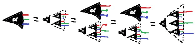
From our starting diagrams, a natural first step is to use the Stitching Rule, to combine together the $M$-diagram and the $i^{th}$ $N$-diagram across the Markov blanket $X$:

Via a couple Bookkeeping steps (add an arrow, reorder complete subgraph) we can rewrite that as

Note that we have $n$ diagrams here (one for each $i$), and the variable ordering $(N,M,X_1,\dots ,X_n)$ respects that diagram for every $i$, so we can Frankenstein all of those diagrams together. $N$ is the root node, $M$ has only $N$ as parent (all diagrams agree on that), and then we take the parent of each $X_i$ from the $i^{th}$ diagram. That yields:

And via one more Bookkeeping operation, we get

as desired.

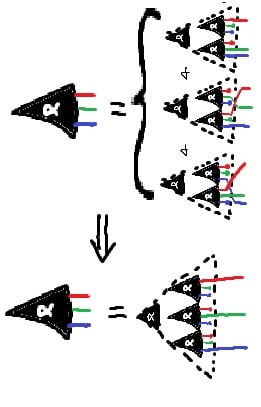
Our full end-to-end proof, presented diagrammatically, looks like this:

Besides readability, one major benefit of this diagrammatic proof is that we can immediately derive approximation bounds for it. We assign a bound to each starting diagram, then just propagate through, using the approximate version of the rule at each step:

As a teaser: one use-case for this particular theorem is that, insofar as the second agent can express things-it-wants in terms of very redundantly represented latent variables (e.g. $N$), it will always be able to express those things in terms of the first agent’s latent variables (i.e. $M$). So, the second agent can express what it wants in terms of the first agent’s internal latent variables. It’s an approach to handling ontological problems, like e.g. The Pointers Problem.

What To Read Next

That concludes our list of rules! This post was written as a prelude to our upcoming post on Natural Latents, which will show a real application of these rules. If you want to build familiarity with the rules, we recommend trying a few exercises in this post, then walking through the proofs in that post (once it’s out), and checking the rules used at each step. There are also several exercises in the appendix of this post, alongside the proofs for the rules.

Appendix: Proofs & Exercises

Re-Rooting Rule for Markov Chains

First, we’ll show that we can move the root node one step to the right.

$\left({\prod }_{i\le k}P\right[X_{i-1}|X_i\left]\right)P\left[X_k\right]\left({\prod }_{k\le i\le n-1}P\right[X_{i+1}|X_i\left]\right)$

$=\left({\prod }_{i\le k}P\right[X_{i-1}|X_i\left]\right)P\left[X_k\right]P\left[X_{k+1}|X_k\right]\left({\prod }_{k+1\le i}P\right[X_{i+1}|X_i\left]\right)$

$=\left({\prod }_{i\le k}P\right[X_{i-1}|X_i\left]\right)P[X_{k+1},X_k]\left({\prod }_{k+1\le i}P\right[X_{i+1}|X_i\left]\right)$

$=\left({\prod }_{i\le k}P\right[X_{i-1}|X_i\left]\right)P\left[X_k|X_{k+1}\right]P\left[X_{k+1}\right]\left({\prod }_{k+1\le i}P\right[X_{i+1}|X_i\left]\right)$

$=\left({\prod }_{i\le k+1}P\right[X_{i-1}|X_i\left]\right)P\left[X_{k+1}\right]\left({\prod }_{k+1\le i}P\right[X_{i+1}|X_i\left]\right)$

Note that the same equations (read backwards) imply we can move the root node one step to the left. Then, by induction, we can move the root node as far as we want in either direction (noting that at either end one of the two products becomes an empty product).

Approximation

The previous proof shows that $\left({\prod }_{i\le k}P\right[X_{i-1}|X_i\left]\right)P\left[X_k\right]\left({\prod }_{k\le i}P\right[X_{i+1}|X_i\left]\right)=\left({\prod }_{i\le k+1}P\right[X_{i-1}|X_i\left]\right)P\left[X_{k+1}\right]\left({\prod }_{k+1\le i}P\right[X_{i+1}|X_i\left]\right)$ for all $X$ (for any distribution). So,

$D_{KL}\left(P\right[X\left]||\right({\prod }_{i\le k}P\left[X_{i-1}|X_i\right]\left)P\right[X_k\left]{\prod }_{k\le i}P\right[X_{i+1}|X_i\left]\right)$

$=D_{KL}\left(P\right[X\left]||\right({\prod }_{i\le k+1}P\left[X_{i-1}|X_i\right]\left)P\right[X_{k+1}\left]{\prod }_{k+1\le i}P\right[X_{i+1}|X_i\left]\right)$

As before, the same equations imply that we can move the root node one step to either the left or right. Then, by induction, we can move the root node as far as we want in either direction, without changing the KL-divergence. 

Exercise

Extend the above proofs to re-rooting of arbitrary trees (i.e. the diagram is a tree). We recommend thinking about your notation first; better choices for notation make working with trees much easier.

Joint Independence Rule: Exercise

The Joint Independence Rule can be proven using the Frankenstein Rule. This is left as an exercise. (And we mean that unironically, it is actually a good simple exercise which will highlight one or two subtle points, not a long slog of tedium as the phrase “left as an exercise” often indicates.)

Bonus exercise: also prove the conditional version of the Joint Independence Rule using the Frankenstein Rule.

Frankenstein Rule

We’ll prove the approximate version, then the exact version follows trivially.

Without loss of generality, assume the order of variables which satisfies all original diagrams is $X_1,\dots ,X_n$. Let $P\left[X\right]={\prod }_{i}P\left[X_i|X_{p{a}^j\left(i\right)}\right]$ be the factorization expressed by diagram $j$, and let $\sigma \left(i\right)$ be the diagram from which the parents of $X_i$ are taken to form the Frankenstein diagram. (The factorization expressed by the Frankenstein diagram is then $P\left[X\right]={\prod }_{i}P\left[X_i|X_{p{a}^{\sigma \left(i\right)}\left(i\right)}\right]$.)

The proof starts by applying the chain rule to the $D_{KL}$ of the Frankenstein diagram:

$D_{KL}\left(P\right[X\left]||{\prod }_{i}P\right[X_i|X_{p{a}^{\sigma \left(i\right)}\left(i\right)}\left]\right)=D_{KL}\left({\prod }_{i}P\right[X_i|X_{<i}||{\prod }_{i}P\left[X_i|X_{p{a}^{\sigma \left(i\right)}\left(i\right)}\right])$

$={\sum }_{i}E\left[D_{KL}\right(P\left[X_i|X_{<i}\right]||P\left[X_i|X_{p{a}^{\sigma \left(i\right)}\left(i\right)}\right]\left)\right]$

Then, we add a few more expected KL-divergences (i.e. add some non-negative numbers) to get:

$\le {\sum }_i{\sum }_{j}E\left[D_{KL}\right(P\left[X_i|X_{<i}\right]||P\left[X_i|X_{p{a}^j\left(i\right)}\right]\left)\right]={\sum }_j{D}_{KL}\left(P\right[X\left]||{\prod }_{i}P\right[X_i|X_{p{a}^j\left(i\right)}\left]\right)$

$\le {\sum }_j{ϵ}_j$

Thus, we have 

$D_{KL}\left(P\right[X\left]||{\prod }_{i}P\right[X_i|X_{p{a}^{\sigma \left(i\right)}\left(i\right)}\left]\right)\le {\sum }_j{D}_{KL}\left(P\right[X\left]||{\prod }_{i}P\right[X_i|X_{p{a}^j\left(i\right)}\left]\right)\le {\sum }_j{ϵ}_j$

Factorization Transfer

Again, we’ll prove the approximate version, and the exact version then follows trivially.

As with the Frankenstein rule, we start by splitting our $D_{KL}$ into a term for each variable:

$D_{KL}\left(P\right[X\left]||Q\right[X\left]\right)={\sum }_{i}E\left[D_{KL}\right(P\left[X_i||X_{<i}\right]||Q\left[X_i||X_{pa\left(i\right)}\right]\left)\right]$

Next, we subtract some more $D_{KL}$’s (i.e. subtract some non-negative numbers) to get:

$\ge {\sum }_i\left(E\right[D_{KL}\left(P\right[X_i||X_{<i}\left]||Q\right[X_i||X_{pa\left(i\right)}\left]\right)]-E[D_{KL}\left(P\right[X_i||X_{pa\left(i\right)}\left]||Q\right[X_i||X_{pa\left(i\right)}\left]\right)\left]\right)$

$={\sum }_{i}E\left[D_{KL}\right(P\left[X_i||X_{<i}\right]||P\left[X_i||X_{pa\left(i\right)}\right]\left)\right]$

$=D_{KL}\left(P\right[X\left]||{\prod }_{i}P\right[X_i||X_{pa\left(i\right)}\left]\right)$

Thus, we have

$D_{KL}\left(P\right[X\left]||Q\right[X\left]\right)\ge D_{KL}\left(P\right[X\left]||{\prod }_{i}P\right[X_i||X_{pa\left(i\right)}\left]\right)$

Stitching

We start with the $X\leftarrow Y\to Z$ condition:

${ϵ}_{\text{blanket}}\ge D_{KL}\left(P\right[X,Y,Z\left]||P\right[X|Y\left]P\right[Y\left]P\right[Z|Y\left]\right)$

$=D_{KL}\left(P\right[X,Y,Z\left]||P\right[X,Y\left]P\right[Z,Y\left]/P\right[Y\left]\right)$

At a cost of at most ${ϵ}_{XY}$, we can replace $P[X,Y]$ with ${\prod }_{i}P\left[\right(X,Y{)}_i|(X,Y{)}_{p{a}^{XY}\left(i\right)}]$ in that expression, and likewise for the $P[Z,Y]$ term. (You can verify this by writing out the $D_{KL}$’s as expected log probabilities.)