Machine learning systems are typically trained to maximize average-case performance. However, this method of training can fail to meaningfully control the probability of tail events that might cause significant harm. For instance, while an artificial intelligence (AI) assistant may be generally safe, it would be catastrophic if it ever suggested an action that resulted in unnecessary large-scale harm.

Current techniques for estimating the probability of tail events are based on finding inputs on which an AI behaves catastrophically. Since the input space is so large, it might be prohibitive to search through it thoroughly enough to detect all potential catastrophic behavior. As a result, these techniques cannot be used to produce AI systems that we are confident will never behave catastrophically.

We are excited about techniques to estimate the probability of tail events that do not rely on finding inputs on which an AI behaves badly, and can thus detect a broader range of catastrophic behavior. We think developing such techniques is an exciting problem to work on to reduce the risk posed by advanced AI systems:

• Estimating tail risk is a conceptually straightforward problem with relatively objective success criteria; we are predicting something mathematically well-defined, unlike instances of eliciting latent knowledge (ELK) where we are predicting an informal concept like "diamond".
• Improved methods for estimating tail risk could reduce risk from a variety of sources, including central misalignment risks like deceptive alignment.
• Improvements to current methods can be found both by doing empirical research, or by thinking about the problem from a theoretical angle.

This document will discuss the problem of estimating the probability of tail events and explore estimation strategies that do not rely on finding inputs on which an AI behaves badly. In particular, we will:

• Introduce a toy scenario about an AI engineering assistant for which we want to estimate the probability of a catastrophic tail event.
• Explain some deficiencies of adversarial training, the most common method for reducing risk in contemporary AI systems.
• Discuss deceptive alignment as a particularly dangerous case in which adversarial training might fail.
• Present methods for estimating the probability of tail events in neural network behavior that do not rely on evaluating behavior on concrete inputs.
• Conclude with a discussion of why we are excited about work aimed at improving estimates of the probability of tail events.

This document describes joint research done with Jacob Hilton, Victor Lecomte, David Matolcsi, Eric Neyman, Thomas Read, George Robinson, and Gabe Wu. Thanks additionally to Ajeya Cotra, Lukas Finnveden, and Erik Jenner for helpful comments and suggestions.

A Toy Scenario

Consider a powerful AI engineering assistant. Write $M$ for this AI system, and $M\left(x\right)$ for the action it suggests given some project description $x$.

We want to use this system to help with various engineering projects, but would like it to never suggest an action that results in large-scale harm, e.g. creating a doomsday device. In general, we define a behavior as catastrophic if it must never occur in the real world.^[1] An input is catastrophic if it would lead to catastrophic behavior.

Assume we can construct a catastrophe detector $C$ that tells us if an action $M\left(x\right)$ will result in large-scale harm. For the purposes of this example, we will assume both that $C$ has a reasonable chance of catching all catastrophes and that it is feasible to find a useful engineering assistant $M$ that never triggers $C$ (see Catastrophe Detectors for further discussion). We will also assume we can use $C$ to train $M$, but that it is prohibitively expensive to use $C$ to filter all of $M$'s outputs after $M$ is trained.^[2]

We are interested in estimating the probability that our model $M$ behaves catastrophically on a particular distribution of inputs^[3]: $P_{x\sim D}\left(C\right(M\left(x\right)\left)\right)$

Deficiencies of Adversarial Training

To reduce the risk of our AI system behaving catastrophically, we could use adversarial training: having a red team attempt to find catastrophic inputs and training $M$ until those inputs are no longer catastrophic.

However, such systems can still behave catastrophically in a range of possible scenarios:

1. The users of an AI system might explore inputs not considered during the adversarial training process and uncover novel catastrophic inputs.
2. Users of a system might specifically search for inputs designed to elicit catastrophic behavior, using more resources than the adversarial training process.^[4]
3. An intelligent AI system may attempt to purposefully avoid acting catastrophically when it suspects it is being trained.

As catastrophic behavior becomes extremely rare, it can be computationally prohibitive for the red team to explore the input space thoroughly enough to find even a single catastrophic input. To determine which AI systems robustly avoid catastrophic behavior, we must be able to estimate the frequency of catastrophic inputs even when they are so rare that we cannot find any such inputs.

Rather than viewing a red team as searching for particular inputs, we can view the red team as defining a process $D$ for producing inputs. We can then ask the question: how likely is the red team to find an input on which the system behaves catastrophically? Equivalently, what is $P_D\left(C\right(M\left(x\right)\left)\right)$? Even if a red team is usually unable to find concrete inputs on which a system behaves catastrophically, the process they use could still have a small probability of success.

The possibility of distributional shift complicates the way in which estimates of the rate of catastrophic behavior can be used to mitigate such behavior, which we discuss in Distributional Shift.

Deliberate Subversion of Adversarial Training

Malign intelligent AI systems might have incentives to pretend to be benign during training so they can cause harm later. Call a system "deceptively aligned" if it is a malign system pretending to be benign.^[5] For example, a deceptively aligned engineering assistant might intentionally avoid suggesting an action that creates a doomsday device during training, but seek such opportunities when they would cause real-world harm. A sufficiently advanced system might be able to maintain this deception even through extensive adversarial training.^[6]

Even if a deceptively aligned model has extremely high accuracy at determining whether it is being adversarially trained, it will likely have some probability of making a mistake. If a deceptive system makes mistakes very rarely, then adversarial training would likely fail to find an input that distinguishes it from a benign model. However, the possibility of these mistakes would result in the deceptive model having a higher probability of behaving catastrophically than its benign counterpart, even if the probability is small in absolute terms (we discuss ways in which this might not be true in Catastrophe Detectors. By estimating the probability of catastrophic behavior, we would be able to distinguish between benign and deceptive systems.

Importantly, our estimates do not need to be perfectly accurate to detect deceptive systems. Catastrophic actions are highly complex, so AI systems cannot randomly stumble into catastrophic actions. Deceptive systems behave catastrophically at much higher rates than their benign counterparts because they sometimes deliberately decide to take catastrophic action. To distinguish between benign and deceptive systems, we would not need to characterize the chance a benign model accidentally acts catastrophically; we would only need to notice that there are some conditions under which a model might deliberately act catastrophically.

A Possible Approach for Estimating Tail Risk

This section an approach for estimating the probability of catastrophic behavior of a neural network. We present several simple methods that represent our overall approach. We are optimistic that this kind of approach can ultimately deliver better risk estimates than can be obtained from conventional red teaming, but in experiments so far we have not surpassed baselines based on importance sampling.^[7]

Consider a neural network $M:X\to Y$, a distribution $D$ over $X$, and a binary event $C:Y\to \{0,1\}$. Our goal is to estimate $P_D\left(C\right(M\left(x\right)\left)\right)$.^[8] For our engineering research assistant example above, $X$ is a project description, $Y$ is a suggested action, and $C$ is our catastrophe detector.

If $P_D\left(C\right(M\left(x\right)\left)\right)$ is very low, then even billions of samples might not contain an $x$ such that $C\left(M\right(x\left)\right)=1$. However, it might still be possible to estimate $P_D\left(C\right(M\left(x\right)\left)\right)$ by identifying structure that suggests $M$ may behave catastrophically on some inputs. For example, suppose $C$ embeds an action $M\left(x\right)$ into some latent space and flags it as catastrophic if it is "too large" in 20 specific directions simultaneously. For each of these directions, we could attempt to identify features in $M$ that would result in the embedding of $M\left(x\right)$ being large in that direction. If each such feature were active with probability $\frac{1}{100}$, then we could estimate the chance that $M\left(x\right)$ is too large in all 20 directions simultaneously as $(\frac{1}{100}{)}^{20}={10}^{-40}$.

Our goal is to develop methods that can reliably detect significant risks of catastrophic behavior by identifying such structure.

Layer-by-layer Activation Modeling

We will present one possible approach to producing estimates of tail events in neural networks based on modeling the distribution of each layer of activations in the network. This approach illustrates one way in which a mechanistic analysis of a model could improve estimates of tail events. However, this particular framework also has a few fundamental flaws, which we discuss in Issues with Layer-by-layer Activation Modeling.

We will assume that $C$ is also a neural network and express the composition of $C$ and $M$ as a single function $C\circ M:X\to \{0,1\}$. This composition is a single function which is $1$ if and only if $x$ is a catastrophic input for $M$. Since $C\circ M$ is itself just a larger neural network, we can express it as the composition of $n$ functions $f_0,f_1,...,f_{n-1}$. Each $f_i$ represents a transition between layers in our model, such as a linear transformation followed by a ReLU activation. We will write $X_i$ for the domain of $f_i$, which is typically equal to $R^k$ for some $k$. More specifically, for input $x$ define:

• $x_0:=x\in X_0$
• $x_{i+1}:=f_i\left(x_i\right)\in X_{i+1}$
• $C\left(M\right(x\left)\right):=x_n\in X_n=\{0,1\}$

Our input distribution $D$ is a distribution over $X_0$. Through the composition of the transition functions $f_i$, $D$ also induces a distribution over $X_1,X_2,...,X_n$. Our general method aims to estimate $P_D\left(C\right(M\left(x\right)\left)\right)$ by approximation these induced distributions over $X_i$ as they flow through the network, from input to output. Each implementation of this method will have two key components:

1. For each layer $i$, we will have a class of distributions $P_i$ over $X_i$ that we will use to model the activations at each layer. Formally, $P_i\subseteq \Delta X_i$.
2. A method to update our model as we progress through layers: given a model $P_i\in P_i$ for layer $i$, we need to determine $P_{i+1}\in P_{i+1}$ for layer $i+1$. Formally, this method is a collection of $n-1$ functions from $P_i\to P_{i+1}$, one for each $i=0,...,n-1$.

With these components in place, we can estimate $P_D\left(C\right(M\left(x\right)\left)\right)$ for any $D\in P_0$ as follows:

1. We begin with $D=P_0\in P_0$, representing the input distribution.
2. We apply our update method repeatedly, generating $P_1\in P_1$, $P_2\in P_2$, up to $P_n\in P_n$.
3. Our estimate of $P_D\left(C\right(M\left(x\right)\left)\right)$ is the probability that $P_n$ assigns to the outcome 1.

Toy Example: Finitely Supported Distributions

If $D$ was finitely supported, then it would be trivial to estimate the probability of catastrophe on $D$, but we can use this example to illustrate some general principles. Let all $P_i$ be the class of finitely supported distributions over the associated spaces $X_i$.

Given a finitely supported distribution $D=P_0$, we can apply $f_1$ to each datapoint to generate the empirical distribution $P_1$, which will be the exact distribution of $x_1$. By repeating this process for all layers, we eventually obtain $P_n$. The probability $P_n$ assigns to $1$ will be the exact frequency of catastrophe on $D$.

This calculation is not helpful for adversarial training; if we cannot find any inputs where a catastrophe occurs, then we also cannot find any finitely supported distribution $D$ with non-zero probability of catastrophe. Instead, we would like to allow a red team to define a broader distribution that puts positive (although potentially very small) probability on catastrophic inputs.

Method 1: Gaussian Distribution

To move beyond empirical evaluations, we can approximate the distributions over activations by multivariate Gaussians. Let $P_i$ be the class of all multivariate Gaussians over the activations $X_i$. Write a normal distribution with mean vector $\mu$ and covariance matrix $\Sigma$ as $N(\mu ,\Sigma )$.

To specify an algorithm, we need to a method for choosing $P_{i+1}$ given $P_i$. In this case, we want to choose the multivariate Gaussian $N({\mu }_{i+1},{\Sigma }_{i+1})$ that best approximates $f_i\left(x_i\right)$ where $x_i\sim N({\mu }_i,{\Sigma }_i)$. A non-linear function distribution is typically no longer Gaussian, so perfect modeling is impossible. Instead, we can use various methods to select $N({\mu }_{i+1},{\Sigma }_{i+1})$ based on different notions of approximation quality.^[9]

A standard notion of approximation quality is the Kullback-Leibler (KL) divergence between $f_i\left(N\right({\mu }_i,{\Sigma }_i\left)\right)$ and $N({\mu }_{i+1},{\Sigma }_{i+1})$. By a well-known "moment matching" theorem of Gaussian distributions, we can minimize $\text{KL}\left(f_i\right(N({\mu }_i,{\Sigma }_i)\left)||N\right({\mu }_{i+1},{\Sigma }_{i+1}\left)\right)$ by setting ${\mu }_{i+1}$ and ${\Sigma }_{i+1}$ to the mean vector and covariance matrix of $f_i\left(N\right({\mu }_i,{\Sigma }_i\left)\right)$.^[10]

This Gaussian approximation allows us to move beyond adversarial training on concrete catastrophic inputs. Instead, we can pick ${\mu }_0$ and ${\Sigma }_0$ to maximize $P_{N({\mu }_0,{\Sigma }_0)}\left(C\right(M\left(x\right)\left)\right)$, then train $M$ to minimize $P_{N({\mu }_0,{\Sigma }_0)}\left(C\right(M\left(x\right)\left)\right)$, hopefully capturing a broader range of catastrophic scenarios.

Method 2: Independent Linear Features

Some authors have attempted to extract meaningful features of a model's computation using sparse auto-encoders (SAEs), which find an overcomplete basis in which the activations are typically sparse. SAEs are typically learned by minimizing an empirical estimate of a reconstruction loss. However, if catastrophic inputs are rare, the SAE's training data is unlikely to contain any catastrophic inputs. As such, we might not learn features that are informative for estimating the probability of catastrophic inputs.

We will describe a modified SAE for which we can analytically calculate the loss over a distribution that includes catastrophic inputs, instead of empirically estimating it with training data. The details of this algorithm can be found here, which we summarize below.

Define a given distribution $P_i\in P_i$ by specifying:

1. $m$ feature vectors $v_1,...,v_m\in X_i$.
2. For each feature $v_j$, a distribution $Q_j$ over $R$ representing how strongly that feature activates.

To generate a single sample from this distribution, we:

1. Sample feature weights $a_j\sim Q_j$ independently.
2. Compute the weighted sum of these features ${\Sigma }_j{a}_j{v}_j$

SAEs are typically learned independently for different layers of a neural network. By contrast, our algorithm will use the features from a layer $X_i$ to learn the features for the next layer $X_{i+1}$. More precisely, we will assume that the activations at layer $i$ are distributed according to $P_i$, and then find the distribution $P_{i+1}$ that minimizes $\text{KL}\left(f_i\right(P_i\left)||P_{i+1}\right))$.

We show that we can analytically compute an bound for this KL divergence by using variational inference.^[11] We can then train to $P_{i+1}$ to minimize this lower bound; the result is a variational autoencoder trained with an objective very similar to the conventional objective for a sparse autoencoder. More details of this bound and an algorithm for calculating it efficiently can be found here.

Because we compute bounds analytically, in principle they can be very sensitive to rare events that would never be detected by sampling. However, because KL divergence is defined as an expectation, this loss function may still incentivize the learning of features that are relevant to the typical behavior of the model and not informative about the tails. For example, a "lethality" feature might be informative about the probability an AI system behaves catastrophically, but almost useless for modeling behavior on typical inputs. To overcome this problem, we would like to replace the KL divergence with a loss function that is more sensitive to distributional differences that affect catastrophe probability. Precisely defining this loss function is one of the major open questions for this approach.

Relation to Other Work

Formalizing the Presumption of Independence

Formalizing the Presumption of Independence studies the problem of estimating the expectation of a circuit through the lens of heuristic estimation. The general framework described above is a particular family of heuristic estimation methods based on modeling the activations of successive layers of a neural network.

Many of the methods we have described are inspired by algorithms for heuristic estimation. Most directly, Method 1 Gaussian Distribution is exactly the covariance propagation algorithm described in appendix D.3. Additionally, Method 2 Independent Linear Features can be thought of as finding a basis for which the presumption of independence approximately applies.

For more examples of methods for heuristic estimation that can potentially be translated into techniques for estimating tail risk in neural networks, see Appendix A of Formalizing the Presumption of Independence.

Mechanistic Interpretability

Mechanistic interpretability is a field of research that aims to understand the inner workings of neural networks. We think such research represents a plausible path towards high-quality estimates of tail risk in neural networks, and many of our estimation methods are inspired by work in mechanistic interpretability.

For example, a mechanistic understanding of a neural network might allow us to identify a set of patterns whose simultaneous activation implies catastrophic behavior. We can then attempt to estimate the probability that all features are simultaneously active by using experiments to collect local data and generalizing it with the presumption of independence.

We also hope that estimating tail risk will require the development of methods for identifying interesting structure in neural networks. If so, then directly estimating tail risk in neural networks might lead to greater mechanistic understanding of how those neural networks behave and potentially automate portions of mechanistic interpretability research.

Relaxed Adversarial Training

Relaxed Adversarial Training (RAT) is a high-level proposal to overcome deficiencies in adversarial training by "relaxing" the problem of finding a catastrophic input. We expect our methods for estimating $P_D\left(C\right(M\left(x\right)\left)\right)$ to be instances of the relaxations required for RAT.

Eliciting Latent Knowledge

In Eliciting Latent Knowledge (ELK), we describe a SmartVault AI trained to take actions so a diamond appears to remain in the room. We are concerned that if the sensors are tampered with, the diamond can be stolen while still appearing safe.

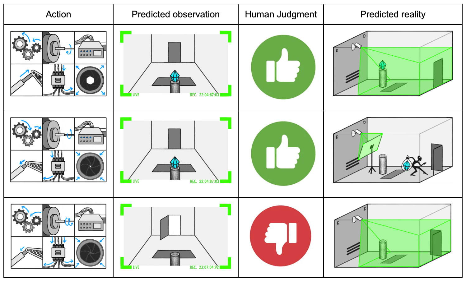
A key difficulty in ELK is the lack of sophisticated tampering attempts on which we can train our model to protect the sensors. In the ELK document, we describe some ways of training models that we hoped would generalize in desirable ways during tampering attempts, but ultimately concluded these methods would not always result in the desired generalization behavior.

Instead of trying to indirectly control generalization, we can attempt to directly measure the quality of generalization by estimating the probability of tampering. We will not have a perfect tampering detector, but even if a robber (or our AI system itself) was skilled at tampering, they might get caught one-in-a-trillion times. Thus, by estimating and minimizing the probability of detectable tampering, we might be able to produce a SmartVault that defends the sensors even with no examples of sophisticated sensor tampering.

More generally, we believe there are deeper connections between methods for estimating tail risk and ELK, which we might explore in a later post.

Conclusion

Contemporary methods for reducing risk from AI systems rely on finding concrete catastrophic inputs. As AI systems become more capable, such methods might not be able to reduce risk down to acceptable levels.

In this document, we have argued that it is both useful and possible to develop approaches for estimating tail risk in neural networks that does not rely on finding concrete catastrophic inputs. We are currently pursuing this problem from both theoretical and empirical angles, and are excited to see others do the same.

We have given a high-level overview of our motivation and approach. In the appendices, we explore various details in more depth:

• In Catastrophe Detectors, we provide a default picture of how to construct a catastrophe detector, and discuss its limitations. We also briefly describe our hope for finding a robust catastrophe detector.
• In Issues with Layer-by-layer Activation Modeling, we overview two major problems with the general estimation framework we discuss in the body, and potential routes for overcoming them.
• In Distributional Shift, we discuss how the possibility of distributional shift complicates the way in which estimates of the rate of catastrophic behavior can be used to mitigate such behavior.
• In Complexity Theoretic Barriers to Accurate Estimates, we discuss why computational barriers to accurate estimates might not prevent us from obtaining estimates "good enough" to mitigate catastrophic behavior.

Appendices

Catastrophe Detectors

In the body, we assume that we can construct a catastrophe detector $C$ that has the following properties:

• $C$ has a reasonable chance of catching everything output by $M$ we would consider a catastrophe.
• It is possible to find a useful $M$ that almost never triggers $C$.

However, we do not currently know how to construct a catastrophe detector with those properties. In this appendix, we will describe the a default picture for how to attempt such a construction, discuss its potential flaws, and briefly overview our hope for why these flaws are surmountable.

Our default picture for how we would attempt to construct such a catastrophe detector is to use a weaker, trusted AI system $M_{weak}$ to examine the suggested action of a stronger system $M$. We could give our weaker system multiple advantages to give it the best chance of catching catastrophic actions:

• We could give $M_{weak}$ more time to think than $M$, so it could examine each portion of the action in detail.
• We could allow $M_{weak}$ to interrogate $M$ about the function of various parts of its action, and do detailed checks for inconsistencies in $M$'s answers.
• We could allow $M_{weak}$ to perform separate experiments to verify $M$'s claims about its actions, and to evaluate whether or not the actions have any side effects.
• $M_{weak}$ could be conservative when evaluating $M$'s action, flagging part of the action it did not understand as potentially catastrophic.

However, even given these advantages, our catastrophe detector $C$ might not have our desired properties:

1. If $M$ is significantly smarter than $M_{weak}$, it might be possible for $M$ to suggest a catastrophic action that $M_{weak}$ will not recognize as such. If $M_{weak}$ merely has a low probability of detecting that such actions are catastrophic, then our estimates will be (potentially poor) approximations to the true probability that $M$ acts catastrophically, but we will still be able to distinguish between deceptive and benign models. If, however, there are catastrophic actions that $M_{weak}$ has no chance of detecting, and $M$ knows that $M_{weak}$ will not be able to detect them, then a deceptive $M$ could act catastrophically while appearing benign.
2. There potentially exist actions that $M_{weak}$ will mistakenly think are catastrophic, and inputs that cause even benign models to produce those actions. For example, contemporary image classifiers are often vulnerable to adversarial attacks that can result in arbitrary misclassification. There might similarly be actions that induce misclassification in $M_{weak}$. If such actions are more common than the probability deceptive models act mistakenly act catastrophically during training, then we would be unable to distinguish between benign and deceptive models.

In the body of this document, we discuss methods for estimating the chance that an AI system violates some specification of catastrophe. We think it is more likely that we fail to find such methods, than that we fail to find a specification of catastrophe that would be valuable to estimate. As such, we have not prioritized research into how we could construct more robust catastrophe specifications.

Our current plan for how to produce such specifications involves increasing the robustness of an imperfect catastrophe detectors using mechanistic anomaly detection. Roughly speaking, we think it should be possible to distinguish between two different "reasons" why an action looked benign:

1. It looked benign because it was benign
2. It looked benign because $M$ carefully selected the action to appear benign.
   This bears resemblance to our plan for how mechanistic anomaly detection will help with ELK, which we discuss in Finding gliders in the game of life.

Issues with Layer-by-layer Activation Modeling

In the body, we present a framework for producing estimates of tail events in a neural network by successively modeling layers of activations. We present this approach because it is easy to communicate and reason about, while still containing the core challenge of producing such estimates. However, we believe the framework to be fundamentally flawed for two reasons:

1. Layer-by-layer modeling forgets too much information
2. Probability distributions over activations are too restrictive

Layer-by-layer modeling forgets too much information

Thanks to Thomas Read for the example used in this section.

When modeling successive layers of activations, we are implicitly forgetting how any particular piece of information was computed. This can result in missing large correlations between activations that are computed in the same way in successive layers.

For example, suppose $h$ is a pseudorandom boolean function that is $1$ on 50% of inputs. Let $x$ be distributed according to some simple distribution $D$. Define the following simple 2 layer neural network:

• $f_1:x\mapsto (x,h(x\left)\right)$
• $f_2:(x,y)\mapsto \left(1\text{iff}h\right(x)==y)$

Since $h\left(x\right)==h\left(x\right)$ definitionally, this network always outputs $1$. However, layer-by-layer activation modeling will give a very poor estimate.

If $h\left(x\right)$ is complex enough, then our activation model will not be able to understand the relationship between $h\left(x\right)$ and $x$, and be forced to treat $h\left(x\right)$ as independent from $x$. So at layer 1, we will model the distribution of activations as $(D,Bern[0.5\left]\right)$, where $Bern\left[0.5\right]$ is 1 with 50% chance and 0 otherwise. Then, for layer 2, we will treat $h\left(x\right)$ and $y$ as independent coin flips, which are equal with 50% chance. So we will estimate $P_D\left(f_2\right(f_1\left(x\right)\left)\right)$ as $0.5$, when it is actually 1.

In general, layer-by-layer activation modeling makes an approximation step at each layer, and implicitly assumes the approximation errors between layers are uncorrelated. However, if layers manipulate information in correlated ways, then approximation errors can also be correlated across layers.

In this case, we hope to be able to notice that $f_1$ and $f_2$ are performing similar computations, and so to realize that the computation done by layer 1 and layer 2 both depend on the value of $h\left(x\right)$. Then, we can model the value of $h\left(x\right)$ as an independent coin flip, and obtain the correct estimate for $P_D\left(f_2\right(f_1\left(x\right)\left)\right)$. This suggests that we must model the entire distribution of activations simultaneously, instead of modeling each individual layer.

Probability distributions over activations are too restrictive

Thanks to Eric Neyman for the example used in this section.

If we model the entire distribution over activations of $M$, then we must do one of two things:

1. Either, the model must only put positive probability on activations which could have been realized by some input
2. Or, the model must put positive probability on an inconsistent set of activations.

Every set of activations actually produced by $M$ is consistent with some input. If we performed consistency checks on $M$, then we would find that every set of activations was always consistent in this way, and the consistency checks would always pass.

If, however, our approximate distribution over $M$'s activations placed positive probability on inconsistent activations, then we would incorrectly estimate the consistency checks as having some chance of failing. In these cases, our estimates could be arbitrarily disconnected from the actual functioning of $M$. So it seems we must strive to put only positive probability on consistent sets of activations.

Only placing positive probability on consistent sets of activations means that our distribution over activations corresponds to some input distribution. This means that our catastrophe estimate will be exact over some input distribution. Unfortunately, this implies our catastrophe estimates will be often be quite poor. For example, suppose we had a distribution over boolean functions with the following properties:

1. a randomly sampled function $f$ is 50% likely to be the constant 0 function, and 50% likely to have a single input where $f\left(x\right)=1$
2. it is computationally hard to tell if $f$ is the all 0 function
   For example, an appropriately chosen distribution over 3-CNFs likely has these properties.

If our input space was of size $N$, then it seems reasonable to estimate a $P\left(f\right)$ as $\frac{1}{2N}$ for randomly sampled $f$. However, since our catastrophe estimate is exact (over some input distribution), it can be non-zero only if $f$ is not the all 0 function. By assumption, it is computationally hard to tell if $f$ is not the all 0 function, so we must generally estimate $P\left(f\right)$ as 0, making it impossible to be "reasonable".

In general, the requirement that our estimate be derived from a logically consistent distribution means we cannot reliably put positive probability on all "reasonable" possibilities. If we wish to be able to produce estimates like $\frac{1}{2N}$, then we must be able to represent logically inconsistent possibilities. However, the possibility of models that do consistency checks means we must place almost no probability on any particular logical inconsistency.

This line of reasoning suggests an overall picture where our estimates are not attached to any particular probability distribution over activations, but rather one where our estimates are derived directly from high-level properties of the distribution. For example, we might instead represent only the moments of the distribution over activations, and our estimate might come from an inconsistent set of moments that cannot come from any possible distribution (but we would not know of any particular inconsistency that was violated).^[12]

Distributional Shift

In Layer-by-layer Activation Modeling, we describe a few methods for estimating the probability of a tail event on a fixed input distribution. However, due to distributional shift, these estimates might be highly uninformative about the true probability our AI systems will act catastrophically "in practice". This problem is not unique to our approach; practitioners of adversarial training also desire to find catastrophic inputs likely to appear "in practice", which might be very different from inputs used to train the AI system.

We have a few rough ideas for constructing distributions that place non-trivial probability on realistic catastrophic inputs:

1. Adding noise to the training distribution produces a wider distribution that is more likely to contain a catastrophic input. In the limit, the uniform distribution over inputs is guaranteed to contain catastrophic inputs should they exist. However, these catastrophic inputs might be highly unrealistic, and represent a small fraction of the catastrophic inputs likely to be encountered "in practice". That being said, lowering the probability an AI system acts catastrophically on random inputs might still make it less likely to act catastrophically in practice.
2. Adversarial training teams might employ various techniques to produce more realistic catastrophic inputs. For instance, they might use other AI systems to modify training inputs, or attempt to directly synthesize catastrophic inputs. Such a strategy is a function from random noise to particular inputs, and thus can also be thought of as distributions over inputs. Instead of sampling from that distribution and hoping it places high enough probability on catastrophic inputs that we will sample one, we can attempt to directly estimate that probability.

Ultimately, however, these mitigations will not detect all instances of deceptive alignment. For example, suppose a deceptively aligned system knows it will encounter a particular input $x$ that is a good opportunity for acting catastrophically. If the adversarial training team does not know about $x$, or merely cannot synthesize $x$, then they will be unable to determine if the system will behave catastrophically.^[13]

In these cases, we hope to detect deceptive alignment by understanding the input distribution "as well as the AI system". Any time the AI system knows that it will encounter some future catastrophic input, we need to incorporate this knowledge into our estimate. This is very related to ELK, and is discussed further in Main hope estimates competitive with the AI system or the training process.

Complexity Theoretic Barriers to Accurate Estimates

It is at least NP-hard to accurately estimate the expectation of a function computable in polynomial time. As such, it is likely infeasible to develop methods for accurately estimating tail events. However, we believe that it is feasible to develop methods that can estimate tail risks accurately enough to detect risks from AI systems deliberately acting catastrophically.

In this appendix, we will first work an example involving 3-SAT to demonstrate some estimation methods that can be applied to problems widely believed to be computationally infeasible to even approximate. Then, we will discuss how we hope to obtain estimates accurate enough to detect risk from AI systems deliberately acting catastrophically by obtaining estimates that are competitive with the AI system or the process used to train it.

3-SAT

A boolean formula is called a 3-CNF if it is formed of an AND of clauses, where each clause is an OR of 3 or less literals. For example, this is a 3-CNF with 3 clauses over 5 variables:

$(x_1\vee \neg x_3\vee x_4)\wedge (\neg x_2\vee x_3\vee \neg x_5)\wedge (x_2\vee \neg x_4\vee x_5)$

We say a given setting of the variables $x_i$ to True or False satisfies the 3-CNF it it makes all the clauses True. 3-SAT is the problem of determining whether there is any satisfying assignment for a 3-CNF. #3-SAT is the problem of determining the number of satisfying assignments for a 3-CNF. Since the number of assignments for a 3-CNF is $2^{\text{number of variables}}$, #3-SAT is equivalent to computing the probability a random assignment is satisfying. The above 3-CNF has 20 satisfying assignments and $2^5=32$ possible assignments, giving a satisfaction probability of $\frac{5}{8}$.

It's widely believed that 3-SAT is computationally hard in the worst case, and #3-SAT is computationally hard to even approximate. However, analyzing the structure of a 3-CNF can allow for reasonable best guess estimates of the number of satisfying assignments.

In the following sections, $F$ is a 3-CNF with $C$ clauses over $n$ variables. We will write $P\left(F\right)$ for the probability a random assignment is satisfying, can be easily computed from the number of satisfying assignments by dividing by $2^n$.

Method 1: Assume clauses are independent

Using brute enumeration over at most 8 possibilities, we can calculate the probability that a clause is satisfied under a random assignment. For clauses involving 3 distinct variables, this will be $\frac{7}{8}$.

If we assume the satisfaction of each clause is independent, then we can estimate $P\left(F\right)$ by multiplying the satisfaction probabilities of each clause. If all the clauses involve distinct variables, this will be $(\frac{7}{8}{)}^C$. We will call this this naive acceptance probability of $F$.

Method 2: Condition on the number of true variables

We say the sign of $x_i$ is positive, and the sign of $\neg x_i$ is negative. If $F$ has a bias in the sign of its literals, then two random clauses are more likely to share literals of the same sign, and thus be more likely to be satisfied on the same assignment. Our independence assumption in method 1 fails to account for this possibility, and thus will underestimate $P\left(F\right)$ in the case where $F$ has biased literals.

We can account for this structure by assuming the clauses of $F$ are satisfied independently conditional on the number of variables assigned true. Instead of computing the probability each clause is true under a random assignment, we can compute the probability under a random assignment where $m$ out of $n$ variables is true. For example, the clause $(x_1\vee \neg x_3\vee x_4)$ will be true on $(\frac{n-3}{m-2})$ possible assignments out of $(\frac{n}{m})$, for a satisfaction probability of $(\frac{n-3}{m-2})/(\frac{n}{m})=\frac{m(m-1)(n-m)}{n(n-1)(n-2)}\approx \frac{m}{n}(1-\frac{m}{n})\frac{m}{n}$, where the latter is the satisfaction probability if each variable was true with independent $\frac{m}{n}$ chance. Multiplying together the satisfaction probabilities of each clause gives us an estimate of $P\left(F\right)$ for a random assignment where $m$ out of $n$ variables are true.

To obtain a final estimate, we take a sum over satisfaction probabilities conditional on $m$ weighted by $\frac{(\frac{n}{m})}{2^n}$, the chance that $m$ variables are true.

Method 3: Linear regression

Our previous estimate accounted for possible average unbalance in the sign of literals. However, even a single extremely unbalanced literal can alter $P\left(F\right)$ dramatically. For example, if $x_i$ appears positively in 20 clauses and negatively in 0, then by setting $x_i$ to true we can form a 3-CNF with 1 fewer variable and 20 fewer clauses that has naive acceptance probability of $2^{N-1}(\frac{7}{8}{)}^{(C-20)}$. $x_i$ will be true with $\frac{1}{2}$ chance, so this represents a significant revision.

We can easily estimate $P\left(F\right)$ in a way that accounts for the balance in any particular literal $x_i$. However, it is not simple to aggregate these estimates into a overall estimate for $P\left(F\right)$.

One approach is to combine these estimates linearly in a way that minimizes some measure of error. For instance, if we wanted to minimize mean-square error, then we would treat each estimate as a feature and combine them using linear regression. If we estimate the covariance of each feature using our naive acceptance probability, then this is equivalent to doing linear regression over the reference class of 3-CNF's where the sign of each literal is flipped uniformly at random. For more details, see section 9.2 of Neyman 2024.

This method produces an estimate for $P\left(F\right)$ that has lower mean-square error over random $F$ than method 2, but lacks other intuitively desirable properties like producing estimates in $[0,1]$. We could clamp our estimate, or attempt to do logistic regression instead, but we will have to trade off between many intuitively desirable properties. Deciding which set of tradeoffs to take requires clarifying what kind of accuracy we want, which in turn depends on downstream applications.

Main hope: estimates competitive with the AI system or the training process

As analogy, suppose we have an AI system $M$ that acts catastrophically whenever the input $x$ is a satisfying assignment to a particular 3-CNF $F$. Accurately estimating the probability $M$ behaves catastrophically is likely computationally infeasible. Nevertheless, we still believe we can obtain estimates that are "good enough" to detect if $M$ poses a catastrophic risk.

If $F$ was a randomly selected 3-CNF, then it is still generally computationally infeasible to tell if there exists a satisfying assignment. However, Method 1 presented above is an exact calculation for the expected value of $P\left(F\right)$ for a randomly selected 3-CNF. Since $F$ was in fact randomly selected, it seems reasonable estimate $P\left(F\right)$ using this "reference class" of random $F$s.

If $F$ was not selected randomly, this will not be a "good enough" estimate. For instance, even if we could calculate the probability of acting catastrophically for a random neural network, treating our trained neural network $M$ as a randomly sampled neural network would produce a terrible estimate for the probability it behaved catastrophically. Similarly, if our training process selected $F$ to have a high satisfaction probability, then treating $F$ as a random 3-CNF would produce a very bad estimate for $P\left(F\right)$.

However, in these cases, there is information we could learn that suggests treating $F$ (or $M$) as a random instance would produce a poor estimate. If we knew how $F$ was selected, then we would know that $F$ was not selected randomly, and so we would know not to treat it as such. Since the training process selected $F$, we have an "existence proof" for a process that is as efficient as the training process that knows how $F$ was selected, and thus has the information necessary to produce a more informed estimate of $F$. Our hope is to produce a parallel "training process" for these more informed estimates by starting with an estimate that assumes $M$ is random, then gradually updating the estimate to incorporate all the information used to produce $M$.

More generally, we hope that if $M$ sometimes deliberately decides to act catastrophically then there is some information that our estimate could incorporate to notice this fact. So if can we use all information that we have available to estimate the probability that $M$ acts catastrophically, then we will be able to reliably distinguish between benign and deceptive AI systems.

---

1. For example, it would be catastrophic to destroy all life on Earth. It would be undesirable, but not catastrophic, for a self-driving car to hit a pedestrian. ↩︎

2. It might also be itself catastrophic to filter M's outputs during high-stakes situations if there is no safe fall-back action. ↩︎

3. It might be difficult to determine whether $M\left(x\right)$ is catastrophic without the input $x$. To be more general, we could also provide $x$ to $C$. Since this does not change any the overall presentation and adds notational burden, we use $C\left(M\right(x\left)\right)$. ↩︎

4. For instance, AI systems are often jailbroken shortly after release, despite developer efforts. ↩︎

5. See Carlsmith 2023 for discussion about how such incentives might arise. ↩︎

6. Even if inputs are indistinguishable between training and deployment, an AI typically spends more time deployed than in training. Thus our AI could behave catastrophically with some constant probability that is low enough to avoid acting catastrophically while being trained, but high enough that it is likely to take a catastrophic action eventually. Section 4.5 of Risks from Learned Optimization makes a similar argument. ↩︎

7. We will release some empirical work on estimating tail events later this year. ↩︎

8. Unfortunately, obtaining accurate estimates of the probability of arbitrary binary functions is computationally infeasible; we discuss such objections in Complexity Theoretic Barriers to Accurate Estimates. ↩︎

9. This problem is well known; for an overview of such methods, see section 8 of Murphy 2023. ↩︎

10. See section 2 of Minka 2013 for the "moment matching" theorem. If $f_i$ is a low-degree polynomial, these values can be computed exactly using Isserlis' Theorem. If $f_i$ involves a ReLU, then we can use a polynomial approximation or estimate it numerically. ↩︎

11. See Chapter 10 of Murphy 2023 for an overview of variational inference. ↩︎

12. The sum of squares algorithm is an example of how such an estimation procedure might look. ↩︎

13. For example, the AI system might pick a cryptographic puzzle it thinks will likely be solved, or make some prediction of what the future will look like based on arcane sociological principles. ↩︎